This article was published as part of the Data Science Blogathon.
Introduction
Clustering is an unsupervised machine learning technique. It is the process of dividing the data set into groups in which members of the same group have similar characteristics. The most widely used clustering algorithms are K-means clustering, hierarchical grouping, density-based grouping, model-based grouping, etc. In this article, we will discuss clustering of K-Means in detail.
Grouping of K-stockings
It is the simplest and most commonly used iterative unsupervised learning algorithm. In this, we randomly initialize the K number of centroids in the data (the number of k is found using the Elbow method to be discussed later in this article) and iterate these centroids until no change occurs in the position of the centroid. Let's go over the steps involved in K means grouping for a better understanding.
1) Select the number of clusters for the dataset (K)
2) Select K number of centroid
3) When calculating Euclidean distance or Manhattan distance, assign points to closest centroid, thus creating K groups
4) Now find the original centroid in each group
5) Reassign the entire data point based on this new centroid, then repeat the step 4 until the centroid position does not change.
Finding the optimal number of clusters is an important part of this algorithm. A commonly used method of finding the optimal value of K is Elbow method.
Elbow method
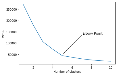
In the elbow method, we are actually varying the number of clusters (K) of 1 a 10. For each value of K, we are calculating WCSS (Sum of the square within the cluster). WCSS is the sum of the squared distance between each point and the centroid in a group. When we graph the WCSS with the value K, the graph looks like a cubit. As the number of clusters increases, the WCSS value will start to decrease. The WCSS value is greater when K = 1. When we analyze the graph, we can see that the graph will change rapidly at one point and, Thus, will create an elbow shape. From this point, the graph begins to move almost parallel to the X axis. The K value corresponding to this point is the optimal K value or an optimal number of clusters.
Now let's implement K-Means clustering using Python.
Implementation
First, we have to import essential libraries.
import numpy as np
import matplotlib.pyplot as plt
import pandas as pd
import sklearn
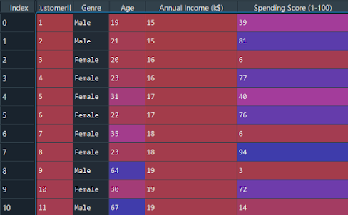
Now let's import the dataset and separate the important features.
dataset = pd.read_csv('Mall_Customers.csv')
X = dataset.iloc[:, [3, 4]].values
We have to find the optimal value of K to group the data. Now we are using the elbow method to find the optimal value of K.
from sklearn.cluster import KMeans
wcss = [] for i in range(1, 11):
    kmeans = KMeans(n_clusters = i, init="k-means++", random_state = 42)
    kmeans.fit(X)
    wcss.append(kmeans.inertia_)
The argument “init” is the method to initialize the centroid. We calculate the WCSS value for each K value. Now we have to plot the WCSS with value K
plt.plot(range(1, 11), wcss)
plt.xlabel('Number of clusters')
plt.ylabel('WCSS')
plt.show(
The graph will be-
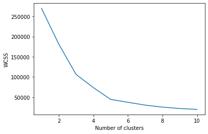
The point where the elbow shape is created is 5, namely, our K-value or an optimal number of clusters is 5. Now let's train the model on the dataset with a number of clusters 5.
kmeans = KMeans(n_clusters = 5, init = "k-means++", random_state = 42)
y_kmeans = kmeans.fit_predict(X)
y_kmeans will be:
array([3, 0, 3, 0, 3, 0, 3, 0, 3, 0, 3, 0, 3, 0, 3, 0, 3, 0, 3, 0, 3, 0,
       3, 0, 3, 0, 3, 0, 3, 0, 3, 0, 3, 0, 3, 0, 3, 0, 3, 0, 3, 0, 3, 1,
       3, 0, 1, 1, 1, 1, 1, 1, 1, 1, 1, 1, 1, 1, 1, 1, 1, 1, 1, 1, 1, 1,
       1, 1, 1, 1, 1, 1, 1, 1, 1, 1, 1, 1, 1, 1, 1, 1, 1, 1, 1, 1, 1, 1,
       1, 1, 1, 1, 1, 1, 1, 1, 1, 1, 1, 1, 1, 1, 1, 1, 1, 1, 1, 1, 1, 1,
       1, 1, 1, 1, 1, 1, 1, 1, 1, 1, 1, 1, 1, 2, 4, 2, 1, 2, 4, 2, 4, 2,
       1, 2, 4, 2, 4, 2, 4, 2, 4, 2, 1, 2, 4, 2, 4, 2, 4, 2, 4, 2, 4, 2,
       4, 2, 4, 2, 4, 2, 4, 2, 4, 2, 4, 2, 4, 2, 4, 2, 4, 2, 4, 2, 4, 2,
       4, 2, 4, 2, 4, 2, 4, 2, 4, 2, 4, 2, 4, 2, 4, 2, 4, 2, 4, 2, 4, 2,
       4, 2])
plt.scatter(X[y_kmeans == 0, 0], X[y_kmeans == 0, 1], s = 60, c="red", label="Cluster1")
plt.scatter(X[y_kmeans == 1, 0], X[y_kmeans == 1, 1], s = 60, c="blue", label="Cluster2")
plt.scatter(X[y_kmeans == 2, 0], X[y_kmeans == 2, 1], s = 60, c="green", label="Cluster3)
plt.scatter(X[y_kmeans == 3, 0], X[y_kmeans == 3, 1], s = 60, c = "violet', label="Cluster4")
plt.scatter(X[y_kmeans == 4, 0], X[y_kmeans == 4, 1], s = 60, c="yellow", label="Cluster5")
plt.scatter(kmeans.cluster_centers_[:, 0], kmeans.cluster_centers_[:, 1], s = 100, c="black", label="Centroids")
plt.xlabel('Annual Income (k$)') plt.ylabel('Spending Score (1-100)') plt.legend()

plt.show()
Graphic:
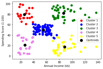
As you can see there 5 groups in total which are displayed in different colors and the centroid of each group is displayed in black.
Complete code
# Importing the libraries
import numpy as np
import matplotlib.pyplot as plt
import pandas as pd # Importing the dataset

X = dataset.iloc[:, [3, 4]].values
dataset = pd.read_csv('Mall_Customers.csv')

from sklearn.cluster import KMeans

# Using the elbow method to find the optimal number of clusters wcss = [] for i in range(1, 11):
 wcss.append(kmeans.inertia_)
 kmeans = KMeans(n_clusters = i, init="k-means++", random_state = 42) kmeans.fit(X) plt.plot(range(1, 11), wcss) plt.xlabel('Number of clusters')

y_kmeans = kmeans.fit_predict(X)

plt.ylabel('WCSS') plt.show() # Training the K-Means model on the dataset kmeans = KMeans(n_clusters = 5, init="k-means++", random_state = 42) y_kmeans = kmeans.fit_predict(X)

# Visualising the clusters
plt.scatter( X[y_kmeans == 1, 0], X[y_kmeans == 1, 1], s = 60, c="blue", label="Cluster2")
plt.scatter( X[y_kmeans == 0, 0], X[y_kmeans == 0, 1], s = 60, c="red", label="Cluster1") plt.scatter( X[y_kmeans == 2, 0], X[y_kmeans == 2, 1], s = 60, c="green", label="Cluster3")
plt.scatter( kmeans.cluster_centers_[:, 0], kmeans.cluster_centers_[:, 1], s = 100, c="black", label="Centroids")
plt.scatter( X[y_kmeans == 3, 0], X[y_kmeans == 3, 1], s = 60, c="violet", label="Cluster4") plt.scatter( X[y_kmeans == 4, 0], X[y_kmeans == 4, 1], s = 60, c="yellow", label="Cluster5") plt.xlabel('Annual Income (k$)') plt.ylabel('Spending Score (1-100)') plt.legend()

plt.show()
Conclution
This is the basic concept of the K-means clustering algorithm in machine learning. In the next articles, we can get more information about different machine learning algorithms.
The media shown in this article is not the property of DataPeaker and is used at the author's discretion.


