Big Data

Analizador de WhatsApp | Análisis de chat grupal de WhatsApp usando Python

Introducción

Hoy en día, una de las plataformas de redes sociales de moda es…. ¿adivina qué? Un único Whatsapp😅. Es una de las plataformas de redes sociales favoritas entre todos nosotros debido a sus características atractivas. Tiene más de 2 mil millones de usuarios en todo el mundo y «según una encuesta, un usuario promedio pasa más de 195 minutos a la semana en WhatsApp». Qué terrible es la declaración anterior. Deje todas estas cosas y entendamos qué significa realmente el analizador de WhatsApp.

WhatsApp Analyzer significa que estamos analizando nuestras actividades grupales de WhatsApp. Realiza un seguimiento de nuestra conversación y analiza cuánto tiempo pasamos o decimos que «desperdiciamos» en WhatsApp. El objetivo de este artículo es proporcionar una guía paso a paso para crear nuestro propio analizador de WhatsApp utilizando Python. Aquí utilicé diferentes bibliotecas de Python que me ayudan a extraer información útil de los datos sin procesar. Aquí elijo mi grupo de WhatsApp oficial de la universidad para analizar el patrón que estaban siguiendo los estudiantes, por lo que en algunas de las instantáneas borro la información de contacto de mis profesores universitarios y mis compañeros, lo siento. Vamos a empezar…

Bibliotecas requeridas:

Regex
Pandas
Matplotlib
Numpy
Seaborn
Fecha y hora
Emoji
Wordcloud
Heatmapz
NLTK
Plotly

Importamos todas estas bibliotecas:

import re
import pandas as pd
import numpy as np
import matplotlib.pyplot as plt
import seaborn as sns
from datetime import *
import datetime as dt
from matplotlib.ticker import MaxNLocator
import regex
import emoji
from seaborn import *
from heatmap import heatmap
from wordcloud import WordCloud , STOPWORDS , ImageColorGenerator
from nltk import *
from plotly import express as px

WhatsApp nos brinda la función de exportar chats, así que exportemos el chat y guardemos el archivo. En el paso 2, crearemos un programa de Python que extraerá la fecha, el nombre de usuario del autor, la hora, los mensajes del archivo de chat exportado y crearemos un marco de datos, y almacenará todos los datos en él. En realidad, la recopilación de datos y la parte de procesamiento previo se tratan en el paso 2 y en los pasos posteriores.

Extraigamos toda la información útil. desde el archivo de chat usando expresiones regulares:

### Python code to extract Date from chat file

def startsWithDateAndTime (s):
patrón = ‘^ ([0-9]+) (/) ([0-9]+) (/) ([0-9][0-9]), ([0-9]+) :([0-9][0-9]) (AM | PM) – ‘
resultado = re.match (patrón, s)
si el resultado:
volver verdadero
falso retorno

### Regex pattern to extract username of Author.

def FindAuthor(s):
    patterns = [
        '([w]+):',                        # First Name
        '([w]+[s]+[w]+):',              # First Name + Last Name
        '([w]+[s]+[w]+[s]+[w]+):',    # First Name + Middle Name + Last Name
        '([+]d{2} d{5} d{5}):',         # Mobile Number (India no.)
        '([+]d{2} d{3} d{3} d{4}):',   # Mobile Number (US no.)
        '([w]+)[u263a-U0001f999]+:',    # Name and Emoji              
    ]
    pattern = '^' + '|'.join(patterns)
    result = re.match(pattern, s)
    if result:
        return True
    return False


### Extracting Date, Time, Author and message from the chat file.

def getDataPoint(line):   
    splitLine = line.split(' - ') 
    dateTime = splitLine[0]
    date, time = dateTime.split(', ') 
    message=" ".join(splitLine[1:])
    if FindAuthor(message): 
        splitMessage = message.split(': ') 
        author = splitMessage[0] 
        message=" ".join(splitMessage[1:])
    else:
        author = None
    return date, time, author, message

### Finally creating a dataframe and storing all data inside that dataframe.

parsedData = [] # List to keep track of data so it can be used by a Pandas dataframe
### Uploading exported chat file
conversationPath="WhatsApp Chat with TE Comp 20-21 Official.txt" # chat file
with open(conversationPath, encoding="utf-8") as fp:
    ### Skipping first line of the file because contains information related to something about end-to-end encryption
    fp.readline() 
    messageBuffer = [] 
    date, time, author = None, None, None
    while True:
        line = fp.readline() 
        if not line: 
            break
        line = line.strip() 
        if startsWithDateAndTime(line): 
            if len(messageBuffer) > 0: 
                parsedData.append([date, time, author, ' '.join(messageBuffer)]) 
            messageBuffer.clear() 
            date, time, author, message = getDataPoint(line) 
            messageBuffer.append(message) 
        else:
            messageBuffer.append(line)
df = pd.DataFrame(parsedData, columns=['Date', 'Time', 'Author', 'Message']) # Initialising a pandas Dataframe.
### changing datatype of "Date" column.
df["Date"] = pd.to_datetime(df["Date"])

Primero, mire nuestro conjunto de datos de recién nacidos:

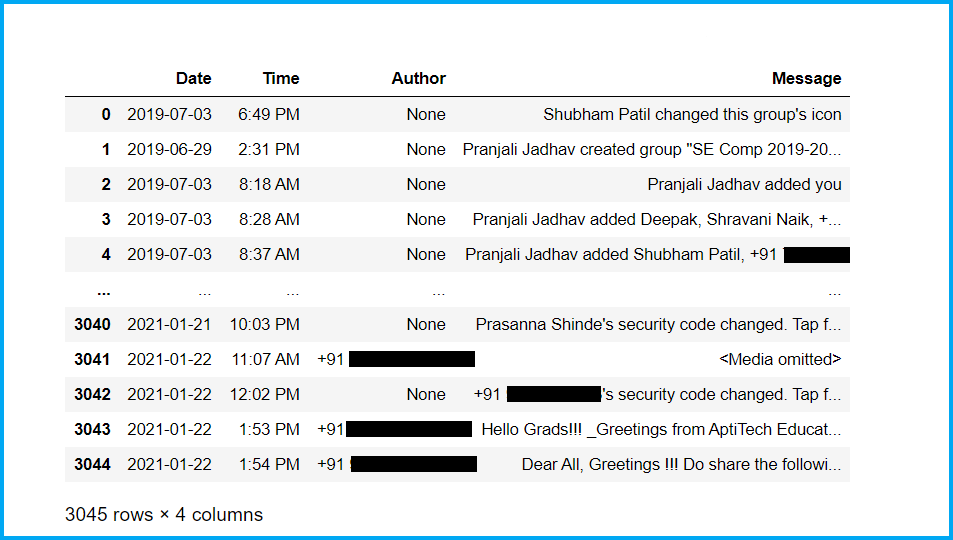
Ahora, verifiquemos la información básica de nuestro conjunto de datos y limpiemos el conjunto de datos:

### Checking shape of dataset.
df.shape
### Checking basic information of dataset
df.info()
### Checking no. of null values in dataset
df.isnull().sum()
### Checking head part of dataset
df.head(50)
### Checking tail part of dataset
df.tail(50)
### Droping Nan values from dataset
df = df.dropna()
df = df.reset_index(drop=True)
df.shape
### Checking no. of authors of group
df['Author'].nunique()
### Checking authors of group
df['Author'].unique()

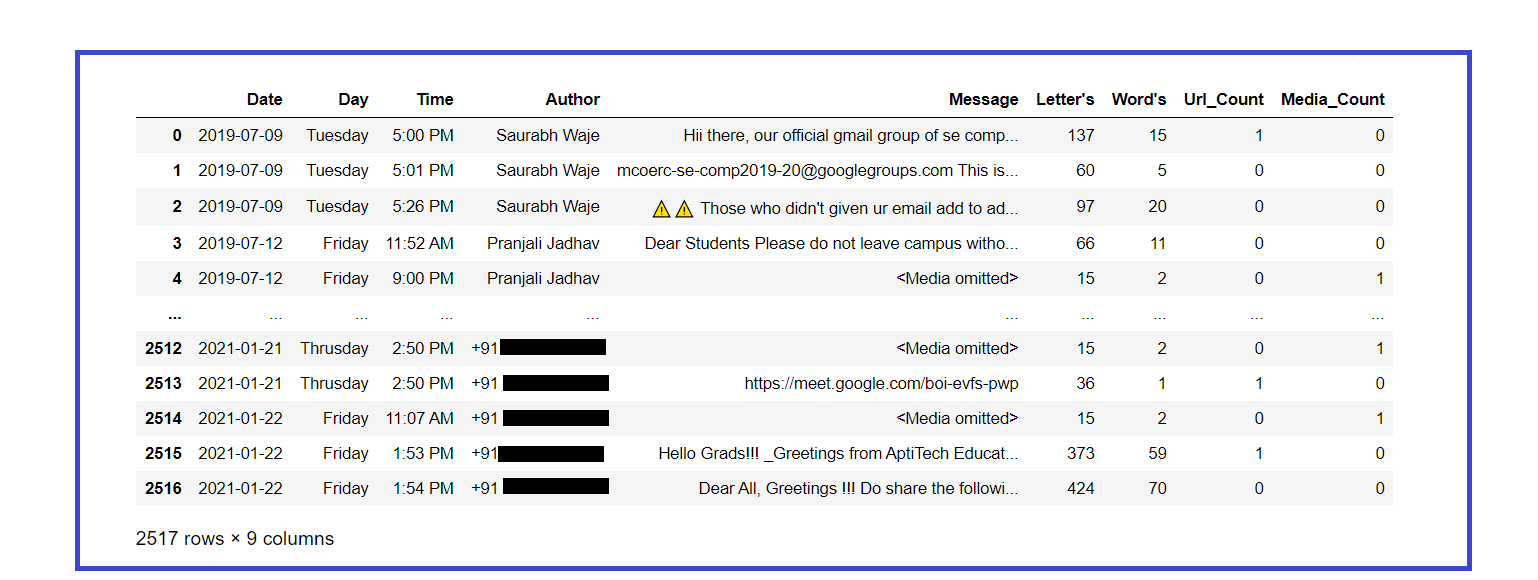
Ahora, procesemos previamente nuestro conjunto de datos e intentemos extraer información útil de él:

### Adding one more column of "Day" for better analysis, here we use datetime library which help us to do this task easily.
weeks = {
0 : 'Monday',
1 : 'Tuesday',
2 : 'Wednesday',
3 : 'Thrusday',
4 : 'Friday',
5 : 'Saturday',
6 : 'Sunday'
}
df['Day'] = df['Date'].dt.weekday.map(weeks)
### Rearranging the columns for better understanding
df = df[['Date','Day','Time','Author','Message']]
### Changing the datatype of column "Day".
df['Day'] = df['Day'].astype('category')
### Looking newborn dataset.
df.head()
### Counting number of letters in each message
df['Letter's'] = df['Message'].apply(lambda s : len(s))
### Counting number of word's in each message
df['Word's'] = df['Message'].apply(lambda s : len(s.split(' ')))
### Function to count number of links in dataset, it will add extra column and store information in it.
URLPATTERN = r'(https?://S+)'
df['Url_Count'] = df.Message.apply(lambda x: re.findall(URLPATTERN, x)).str.len()
links = np.sum(df.Url_Count)
### Function to count number of media in chat.
MEDIAPATTERN = r'<Media omitted>'
df['Media_Count'] = df.Message.apply(lambda x : re.findall(MEDIAPATTERN, x)).str.len()
media = np.sum(df.Media_Count)
### Looking updated dataset
df

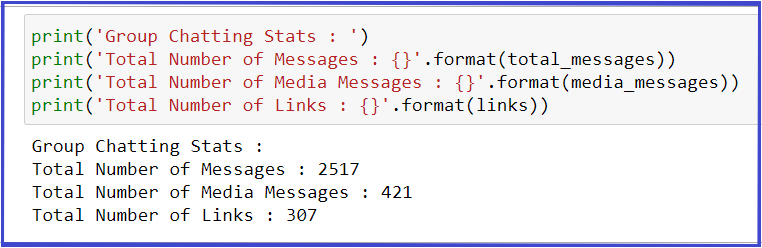
Extraer estadísticas básicas del conjunto de datos:

total_messages = df.shape[0]
media_messages = df[df['Message'] == '<Media omitted>'].shape[0]
links = np.sum(df.Url_Count)
print('Group Chatting Stats : ')
print('Total Number of Messages : {}'.format(total_messages))
print('Total Number of Media Messages : {}'.format(media_messages))
print('Total Number of Links : {}'.format(links))

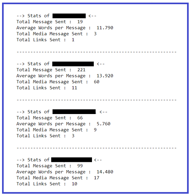
Extrayendo estadísticas básicas de cada usuario:

l = df.Author.unique()
for i in range(len(l)):
  ### Filtering out messages of particular user
  req_df = df[df["Author"] == l[i]]
  ### req_df will contain messages of only one particular user
  print(f'--> Stats of {l[i]} <-- ')
  ### shape will print number of rows which indirectly means the number of messages
  print('Total Message Sent : ', req_df.shape[0])
  ### Word_Count contains of total words in one message. Sum of all words/ Total Messages will yield words per message
  words_per_message = (np.sum(req_df['Word's']))/req_df.shape[0]
  w_p_m = ("%.3f" % round(words_per_message, 2))  
  print('Average Words per Message : ', w_p_m)
  ### media conists of media messages
  media = sum(req_df["Media_Count"])
  print('Total Media Message Sent : ', media)
  ### links consist of total links
  links = sum(req_df["Url_Count"])   
  print('Total Links Sent : ', links)   
  print()
  print('----------------------------------------------------------n')

Creemos una nube de palabras con las palabras más utilizadas en el chat:

### Word Cloud of mostly used word in our Group
text = " ".join(review for review in df.Message)
wordcloud = WordCloud(stopwords=STOPWORDS, background_color="white").generate(text)
  ### Display the generated image:
plt.figure( figsize=(10,5))
plt.imshow(wordcloud, interpolation='bilinear')
plt.axis("off")
plt.show()

Imprimamos el no total. de mensajes enviados por cada usuario:

### Creates a list of unique Authors
l = df.Author.unique()
for i in range(len(l)):
  ### Filtering out messages of particular user
  req_df = df[df["Author"] == l[i]]
  ### req_df will contain messages of only one particular user
  print(l[i],'  ->  ',req_df.shape[0])

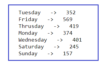
Imprimamos el total de mensajes enviados cada día de la semana:

l = df.Day.unique()
for i in range(len(l)):
  ### Filtering out messages of particular user
  req_df = df[df["Day"] == l[i]]
  ### req_df will contain messages of only one particular user
  print(l[i],'  ->  ',req_df.shape[0])

Finalmente, hemos extraído suficiente información de texto del archivo de chat, ahora comencemos la parte de Visualización de datos que nos ayudará para un mejor análisis y comprensión de todo el análisis que hemos realizado en nuestro archivo de chat exportado. En el lugar de los números de contacto, he usado alfabetos por motivos de seguridad, lo siento mucho.

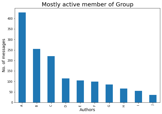
Veamos quién es el autor más activo del grupo:

### Mostly Active Author in the Group
plt.figure(figsize=(9,6))
mostly_active = df['Author'].value_counts()
### Top 10 peoples that are mostly active in our Group is : 
m_a = mostly_active.head(10)
bars = ['A','B','C','D','E','F','G','H','I','J']
x_pos = np.arange(len(bars))
m_a.plot.bar()
plt.xlabel('Authors',fontdict={'fontsize': 14,'fontweight': 10})
plt.ylabel('No. of messages',fontdict={'fontsize': 14,'fontweight': 10})
plt.title('Mostly active member of Group',fontdict={'fontsize': 20,'fontweight': 8})
plt.xticks(x_pos, bars)
plt.show()

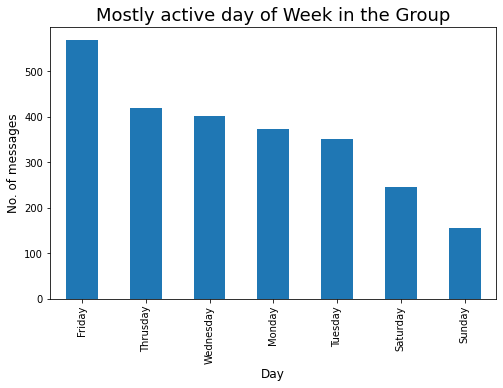
Veamos el día mayormente activo en una semana:

### Mostly Active day in the Group
plt.figure(figsize=(8,5))
active_day = df['Day'].value_counts()
### Top 10 peoples that are mostly active in our Group is : 
a_d = active_day.head(10)
a_d.plot.bar()
plt.xlabel('Day',fontdict={'fontsize': 12,'fontweight': 10})
plt.ylabel('No. of messages',fontdict={'fontsize': 12,'fontweight': 10})
plt.title('Mostly active day of Week in the Group',fontdict={'fontsize': 18,'fontweight': 8})
plt.show()

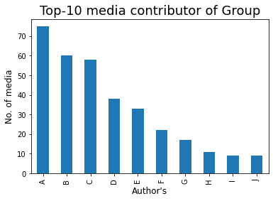
Veamos el contribuyente de medios Top-10 en el grupo:

### Top-10 Media Contributor of Group
mm = df[df['Message'] == '<Media omitted>']
mm1 = mm['Author'].value_counts()
bars = ['A','B','C','D','E','F','G','H','I','J']
x_pos = np.arange(len(bars))
top10 = mm1.head(10)
top10.plot.bar()
plt.xlabel('Author's',fontdict={'fontsize': 12,'fontweight': 10})
plt.ylabel('No. of media',fontdict={'fontsize': 12,'fontweight': 10})
plt.title('Top-10 media contributor of Group',fontdict={'fontsize': 18,'fontweight': 8})
plt.xticks(x_pos, bars)
plt.show()

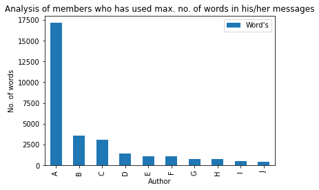
Las palabras son, por supuesto, el arma más poderosa del mundo, así que veamos quién tiene esta poderosa arma en el grupo😅:

max_words = df[['Author','Word's']].groupby('Author').sum()
m_w = max_words.sort_values('Word's',ascending=False).head(10)
bars = ['A','B','C','D','E','F','G','H','I','J']
x_pos = np.arange(len(bars))
m_w.plot.bar(rot=90)
plt.xlabel('Author')
plt.ylabel('No. of words')
plt.title('Analysis of members who has used max. no. of words in his/her messages')
plt.xticks(x_pos, bars)
plt.show()

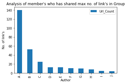
Veamos el autor Top-10 que ha compartido el número máximo. de enlaces en el grupo:

### Member who has shared max numbers of link in Group 
max_words = df[['Author','Url_Count']].groupby('Author').sum()
m_w = max_words.sort_values('Url_Count',ascending=False).head(10)
bars = ['A','B','C','D','E','F','G','H','I','J']
x_pos = np.arange(len(bars))
m_w.plot.bar(rot=90)
plt.xlabel('Author')
plt.ylabel('No. of link's')
plt.title('Analysis of member's who has shared max no. of link's in Group')
plt.xticks(x_pos, bars)
plt.show()

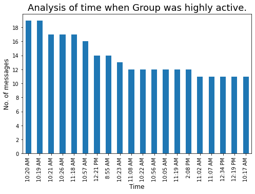
Veamos la hora cada vez que el grupo estuvo muy activo:

### Time whenever our group is highly active
plt.figure(figsize=(8,5))
t = df['Time'].value_counts().head(20)
tx = t.plot.bar()
tx.yaxis.set_major_locator(MaxNLocator(integer=True))  #Converting y axis data to integer
plt.xlabel('Time',fontdict={'fontsize': 12,'fontweight': 10})
plt.ylabel('No. of messages',fontdict={'fontsize': 12,'fontweight': 10})
plt.title('Analysis of time when Group was highly active.',fontdict={'fontsize': 18,'fontweight': 8})
plt.show()

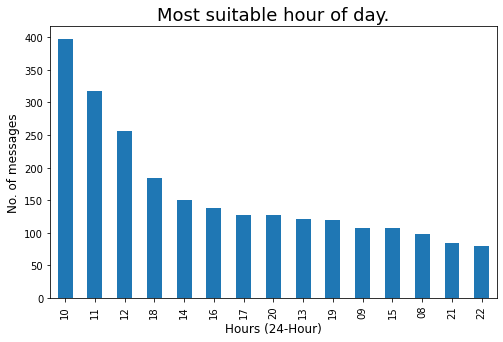
La conversión de formato de 12 horas a 24 horas nos ayudará a realizar un mejor análisis:

lst = []
for i in df['Time'] :
out_time = datetime.strftime(datetime.strptime(i,"%I:%M %p"),"%H:%M")
lst.append(out_time)
df['24H_Time'] = lst
df['Hours'] = df['24H_Time'].apply(lambda x : x.split(':')[0])

Revisemos la hora más adecuada del día cuando haya más posibilidades de obtener una respuesta de los miembros del grupo:

### Most suitable hour of day, whenever there will more chances of getting responce from group members.
plt.figure(figsize=(8,5))
std_time = df['Hours'].value_counts().head(15)
s_T = std_time.plot.bar()
s_T.yaxis.set_major_locator(MaxNLocator(integer=True))  #Converting y axis data to integer
plt.xlabel('Hours (24-Hour)',fontdict={'fontsize': 12,'fontweight': 10})
plt.ylabel('No. of messages',fontdict={'fontsize': 12,'fontweight': 10})
plt.title('Most suitable hour of day.',fontdict={'fontsize': 18,'fontweight': 8})
plt.show()

Creemos una nube de palabras de los 10 miembros más activos:

active_m = [list of Top-10 highly active members]
for i in range(len(active_m)) :
    # Filtering out messages of particular user
    m_chat = df[df["Author"] == active_m[i]]
    print(f'--- Author :  {active_m[i]} --- ')
    # Word Cloud of mostly used word in our Group
    msg = ' '.join(x for x in m_chat.Message)
    wordcloud = WordCloud(stopwords=STOPWORDS, background_color="white").generate(msg)
    plt.figure(figsize=(10,5))
    plt.imshow(wordcloud, interpolation='bilinear')
    plt.axis("off")
    plt.show()
    print('____________________________________________________________________________________n')

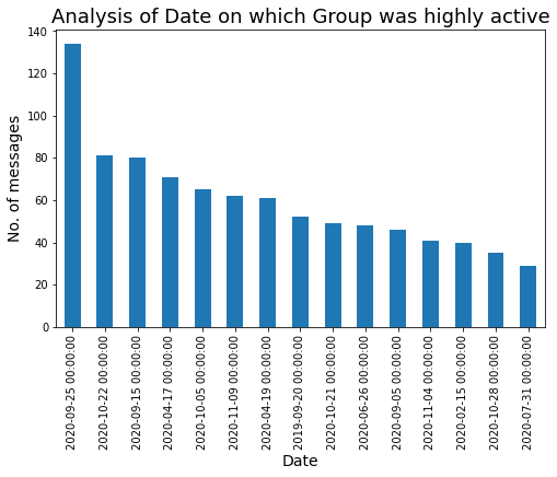
Veamos la fecha en la que nuestro grupo estuvo muy activo:

### Date on which our Group was highly active.
plt.figure(figsize=(8,5))
df['Date'].value_counts().head(15).plot.bar()
plt.xlabel('Date',fontdict={'fontsize': 14,'fontweight': 10})
plt.ylabel('No. of messages',fontdict={'fontsize': 14,'fontweight': 10})
plt.title('Analysis of Date on which Group was highly active',fontdict={'fontsize': 18,'fontweight': 8})
plt.show()

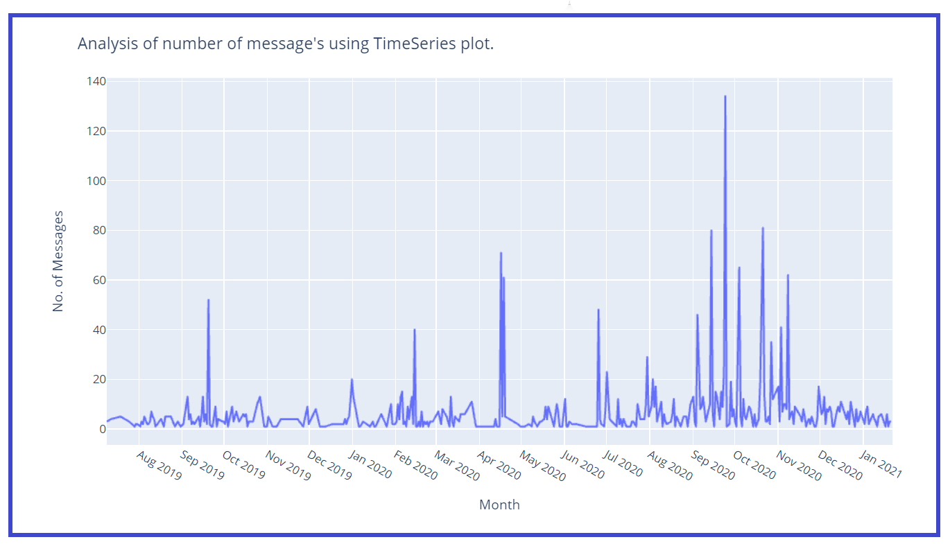
Creemos una gráfica de series de tiempo wrt no. de mensajes:

z = df['Date'].value_counts() 
z1 = z.to_dict() #converts to dictionary
df['Msg_count'] = df['Date'].map(z1)
### Timeseries plot 
fig = px.line(x=df['Date'],y=df['Msg_count'])
fig.update_layout(title="Analysis of number of message"s using TimeSeries plot.',
                  xaxis_title="Month",
                  yaxis_title="No. of Messages")
fig.update_xaxes(nticks=20)
fig.show()

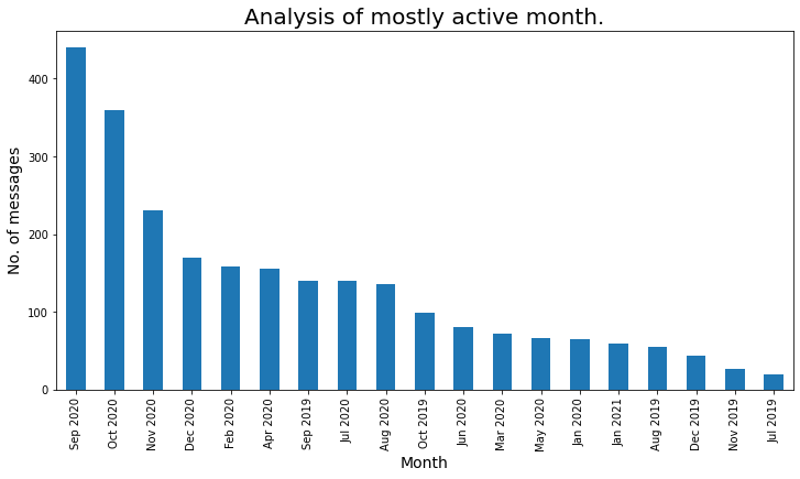
Creemos una columna separada para Mes y Año para un mejor análisis:

df['Year'] = df['Date'].dt.year
df['Mon'] = df['Date'].dt.month
months = {
     1 : 'Jan',
     2 : 'Feb',
     3 : 'Mar',
     4 : 'Apr',
     5 : 'May',
     6 : 'Jun',
     7 : 'Jul',
     8 : 'Aug',
     9 : 'Sep',
    10 : 'Oct',
    11 : 'Nov',
    12 : 'Dec'
}
df['Month'] = df['Mon'].map(months)
df.drop('Mon',axis=1,inplace=True)

Veamos el mes mayormente activo:

### Mostly Active month 
plt.figure(figsize=(12,6))
active_month = df['Month_Year'].value_counts()
a_m = active_month
a_m.plot.bar()
plt.xlabel('Month',fontdict={'fontsize': 14,'fontweight': 10})
plt.ylabel('No. of messages',fontdict={'fontsize': 14,'fontweight': 10})
plt.title('Analysis of mostly active month.',fontdict={'fontsize': 20,
        'fontweight': 8})
plt.show()

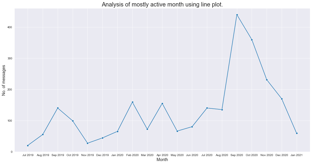
Analicemos el mes más activo usando un diagrama de líneas:

z = df['Month_Year'].value_counts() 
z1 = z.to_dict() #converts to dictionary
df['Msg_count_monthly'] = df['Month_Year'].map(z1)
plt.figure(figsize=(18,9))
sns.set_style("darkgrid")
sns.lineplot(data=df,x='Month_Year',y='Msg_count_monthly',markers=True,marker="o")
plt.xlabel('Month',fontdict={'fontsize': 14,'fontweight': 10})
plt.ylabel('No. of messages',fontdict={'fontsize': 14,'fontweight': 10})
plt.title('Analysis of mostly active month using line plot.',fontdict={'fontsize': 20,'fontweight': 8})
plt.show()

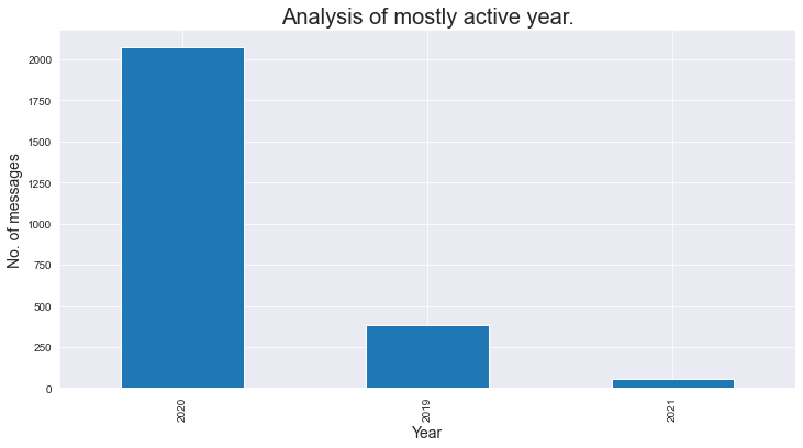
Revisemos el mensaje total por año:

### Total message per year
### As we analyse that the group was created in mid 2019, thats why number of messages in 2019 is less.
plt.figure(figsize=(12,6))
active_month = df['Year'].value_counts()
a_m = active_month
a_m.plot.bar()
plt.xlabel('Year',fontdict={'fontsize': 14,'fontweight': 10})
plt.ylabel('No. of messages',fontdict={'fontsize': 14,'fontweight': 10})
plt.title('Analysis of mostly active year.',fontdict={'fontsize': 20,'fontweight': 8})
plt.show()

Usemos un mapa de calor y analicemos la hora del día con gran actividad:

df2 = df.groupby(['Hours', 'Day'], as_index=False)["Message"].count()
df2 = df2.dropna()
df2.reset_index(drop = True,inplace = True)
### Analysing on which time group is mostly active based on hours and day.
analysis_2_df = df.groupby(['Hours', 'Day'], as_index=False)["Message"].count()
### Droping null values
analysis_2_df.dropna(inplace=True)
analysis_2_df.sort_values(by=['Message'],ascending=False)
day_of_week = ['Monday', 'Tuesday', 'Wednesday', 'Thrusday', 'Friday', 'Saturday', 'Sunday']
plt.figure(figsize=(15,8))
heatmap(
    x=analysis_2_df['Hours'],
    y=analysis_2_df['Day'],
    size_scale = 500,
    size = analysis_2_df['Message'], 
    y_order = day_of_week[::-1],
    color = analysis_2_df['Message'], 
    palette = sns.cubehelix_palette(128)
)
plt.show()

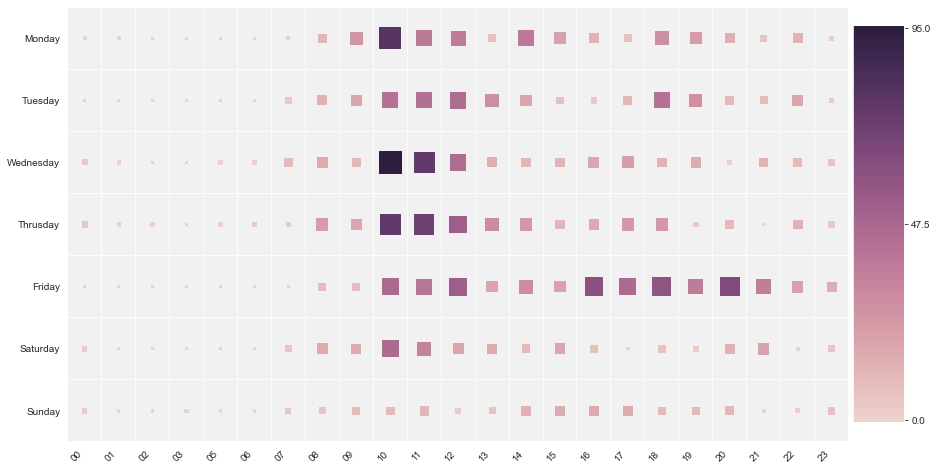
A partir del mapa de calor anterior, analizamos que el «lunes» entre las 10:00 y las 10:59, nuestro grupo fue
muy activo, de manera similar el «miércoles» entre las 10:00 y las 10:59, nuestro grupo estaba
altamente activo. Entre las 00:00 y las 08:00 el grupo estuvo menos activo.

Nota final:

Espero que este artículo realmente te ayude a crear tu propio analizador de chat de WhatsApp y analizar el patrón en el grupo.

Espero que hayas disfrutado de este artículo. ¿Cualquier pregunta? ¿Me he perdido algo? Por favor comuníquese conmigo en mi LinkedIn. Y finalmente, … no hace falta decir,