Source: https://www.serokell.io
In the picture above, you can see emails are classified as spam or not. Then, is an example of classification (binary classification).
1. Logistic regression
2. Bayes ingenuo
3. K-Nearest Neighbors
5. Decisions Tree
We will see all the algorithms with a small code applied in the iris data set that is used for classification tasks. The data set has 150 instances (rows), 4 features (columns) and does not contain any null value. There is 3 classes in iris dataset:
– Silky Iris
– Iris Versicolor
– Iris Virginica
It is a very basic but important classification algorithm in machine learning that uses one or more independent variables to establish a result. Logistic regression attempts to find the link that best fits between the dependent variable and a set of independent variables. The line that best fits in this algorithm looks like the S shape, as the picture shows.
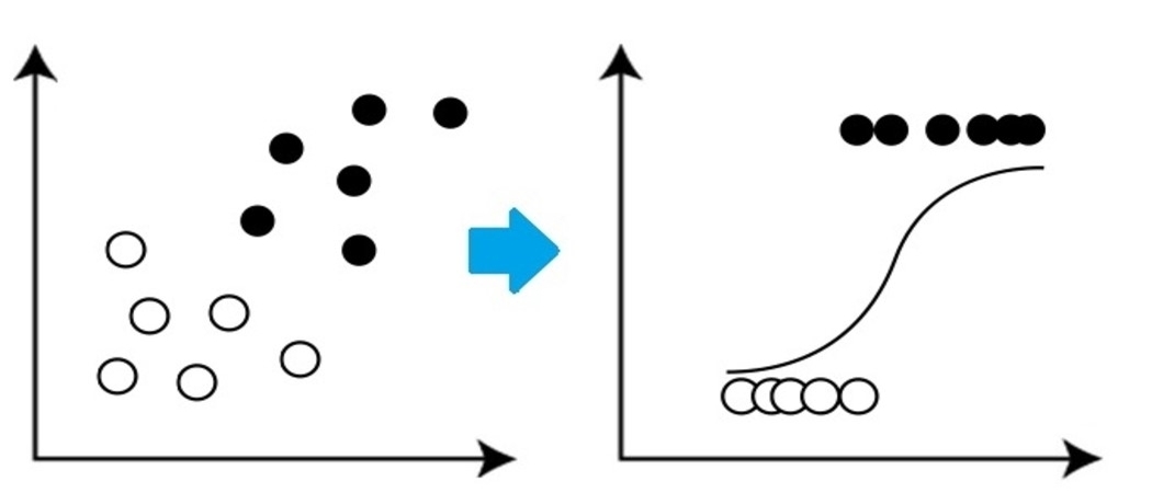
Source: https://www.equiskill.com
Pros:
- It is a very simple and efficient algorithm.
- Low variance.
- Provides probability observation score.
Cons:
- Bad driving a great number of categorical characteristics.
- Assume that the data are free of missing values and that the predictors are independent of each other.
Example:
from sklearn.datasets import load_iris
from sklearn.linear_model import LogisticRegression
X, y = load_iris()
LR_classifier = LogisticRegression(random_state=0)
LR_classifier.fit(X, Y)
LR_classifier.predict(X[:3, :])
Production:
array([0, 0, 0])
It predicted 0 class for all 3 tests given to predict function.
2. Bayes ingenuo
Naive Bayes se basa en Teorema de bayes which gives an assumption of independence between predictors. This classifier assumes that the presence of a particular characteristic in one class is not related to the presence of any other
characteristic / variable.
Naive Bayes classifiers are of three types: Multinomial Naive Bayes, Bernoulli Naive Bayes, Gaussian Naive Bayes.
Pros:
- This algorithm works very fast.
- It can also be used to solve multi-class prediction problems., since it is quite useful with them.
- This classifier performs better than other models with less training data if the assumption of independence of the characteristics is maintained..
Cons:
- Assumes
that all functions are independent. Although it may sound great in
theory, But in real life, no one can find a set of independent characteristics.
Example:
from sklearn.datasets import load_iris
from sklearn.model_selection import train_test_split
from sklearn.naive_bayes import GaussianNB
X, y = load_iris(return_X_y=True)
X_train, X_test, y_train, y_test = train_test_split(X, Y, test_size=0.25, random_state=142)
Naive_Bayes = GaussianNB()
Naive_Bayes.fit(X_train, y_train)
prediction_results = Naive_Bayes.predict(X_test)
print(prediction_results)
Production:
array([0, 1, 1, 2, 1, 1, 0, 0, 2, 1, 1, 1, 2, 0, 1, 0, 2, 1, 1, 2, 2, 1,0, 1, 2, 1, 2, 2, 0, 1, 2,
     1, 2, 1, 2, 2, 1, 2])
These are the classes predicted for X_test data by our naive Bayes model.
3. Nearest neighbor algorithm K
You must have heard of a popular saying:
“Birds of a feather flock together.”
KNN works on the same principle. Classify the new data points based on the class of the most data points between neighbor K, where K is the number of neighbors to consider. KNN captures the idea of similarity (sometimes called distance,
proximity or closeness) with some basic math distance formulas like Euclidean distance, distance from Manhattan, etc.
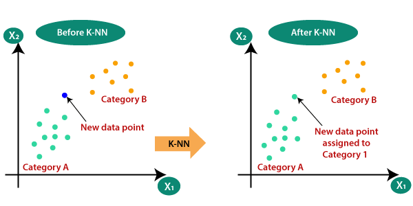
Source: https://www.javatpoint.com
Select the correct value for K
To choose the appropriate K for the data you want to train, run KNN algorithm multiple times with different K values and choose that K value which reduces the amount of errors in the unseen data.
Pros:
- KNN is simple and easy to implement.
- No need to create a model, adjust various parameters or make additional assumptions like some of the other classification algorithms.
- Can be used for classification, regression and search. Then, it is flexible.
- The algorithm becomes significantly slower as the number of examples increases and / or predictors / independent variables.
from sklearn.neighbors import KNeighborsClassifier
X_train, X_test, y_train, y_test = train_test_split(X, Y, test_size=0.25, random_state=142)
knn = KNeighborsClassifier(n_neighbors=3)
knn.fit(X_train, y_train)
prediction_results = knn.predict(X_test[:5,:)
print(prediction_results)
Production:
array([0, 1, 1, 2, 1])
We predicted our results for 5 sample rows. Hence we have 5 results in array.
4. SVM
SVM stands for Support Vector Machine. This is a supervised machine learning algorithm that is used very frequently for classification and regression challenges. Despite this, mainly used in classification problems. The basic concept of Support Vector Machine and how it works can be better understood with this simple example. Then, imagine you have two labels: green and blue, and our data has two characteristics: X Y Y. We want a classifier that, given a couple of (x, Y) coordinates, outputs if it is verde O blue. Plot the labeled training data on a plane and then try to find a plane (the hyperplane of dimensions increases) which segregates the data points of both colors very clearly.
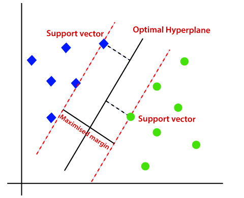
Source: https://www.javatpoint.com
But this is the case for linear data. But, What if the data is not linear, then use the kernel trick? Then, to handle this, we increase the dimension, this brings data into space and now the data becomes linearly separable into two groups.
Pros:
- SVM works relatively well when there is a clear margin of separation between classes.
- SVM is more effective in large spaces.
Cons:
- SVM is not suitable for large data sets.
- SVM does not work very well when the dataset has more noise, In other words, when target classes overlap. Then, needs to be handled.
Example:
from sklearn import svm
svm_clf = svm.SVC()
X_train, X_test, y_train, y_test = train_test_split(X, Y, test_size=0.25, random_state=142)
svm_clf.fit(X_train, y_train)
prediction_results = svm_clf.predict(X_test[:7,:])
print(prediction_results)
Production:
array([0, 1, 1, 2, 1, 1, 0])
5.Decision tree
The decision tree is one of the most widely used machine learning algorithms. They are used for classification and regression problems. Decision trees mimic human-level thinking, so it is very easy to understand the data and make good intuitions and interpretations. In reality, make you see the logic of the data to interpret it. Decision trees are not like black box algorithms like SVM, neural networks, etc.
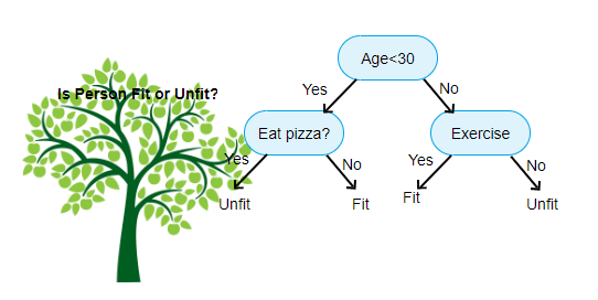
Source: https://www.aitimejournal.com
As an example, whether we classify a person as fit or unfit, the decision tree looks a bit like this in the picture.
Then, in summary, A decision tree is a tree where each node represents a
characteristic / attribute, each branch represents a decision, a ruler and each sheet represents a result. This result can be of categorical or continuous value. Categorical in case of classification and continuous in case of regression applications.
Pros:
- Compared to other algorithms, decision trees require less effort for data preparation throughout preprocessing.
- They also don't require data normalization or scaling.
- The model developed in the decision tree is very intuitive and easy to explain to both technical teams and stakeholders..
Cons:
- If even a small change is made to the data, that can lead to a big change in the decision tree structure causing instability.
- Sometimes, calculation can be much more complex compared to other algorithms.
- Decision trees usually take longer to train the model.
Example:
from sklearn import tree
dtc = tree.DecisionTreeClassifier()
X_train, X_test, y_train, y_test = train_test_split(X, Y, test_size=0.25, random_state=142)
dtc.fit(X_train, y_train)
prediction_results = dtc.predict(X_test[:7,:])
print(prediction_results)
Production:
array([0, 1, 1, 2, 1, 1, 0])
Final notes
These are the 5 most popular ranking algorithms, there are many more and also advanced algorithms. Explore them further. Let's connect LinkedIn
Thanks for reading if you got here 🙂
The media shown in this post is not the property of DataPeaker and is used at the author's discretion.


