
This article was published as part of the Data Science Blogathon
Introduction
In this article, aprenderemos cómo una de las técnicas de deep learningDeep learning, A subdiscipline of artificial intelligence, relies on artificial neural networks to analyze and process large volumes of data. This technique allows machines to learn patterns and perform complex tasks, such as speech recognition and computer vision. Its ability to continuously improve as more data is provided to it makes it a key tool in various industries, from health... utilizadas para encontrar la precisión de Breast Cancer Data Set, but i know most techs don't know what we're talking about, we'll start from the basics and then move on to our topic. First, we will do a brief introduction to deep learning and then, ¿qué es la red neuronalNeural networks are computational models inspired by the functioning of the human brain. They use structures known as artificial neurons to process and learn from data. These networks are fundamental in the field of artificial intelligence, enabling significant advancements in tasks such as image recognition, Natural Language Processing and Time Series Prediction, among others. Their ability to learn complex patterns makes them powerful tools.. artificial?
What is deep learning?
If we talk about deep learning, just understand that it is a subset or subpart of machine learning. We can say that deep learning is an AI function that mimics the human brain and processes that data and creates patterns to use in decision making.
Deep learning is the kind of machine learning that is kind of like the human brain. Uses a multi-layered structure of algorithms called neural networks. Their algorithms try to copy the data that humans would be analyzing with a certain logical structure. Also known as deep neural network or deep neural learning.
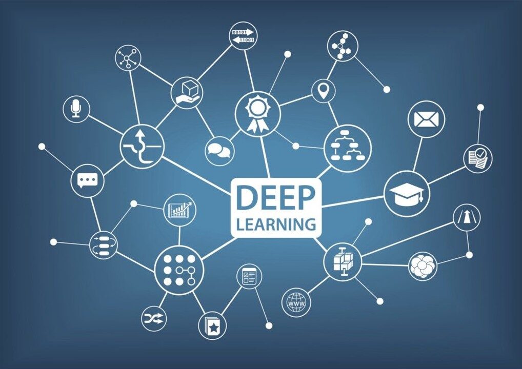
In deep learning there is a concept called Artificial Neural Network which we will briefly discuss below.:
Red neuronal artificial
As the name suggests artificial neural network, is the network of artificial neurons. Refers to a biologically inspired model in the brain. We can say that it is usually a computational network based on biological neural networks that build the structure of the human brain.
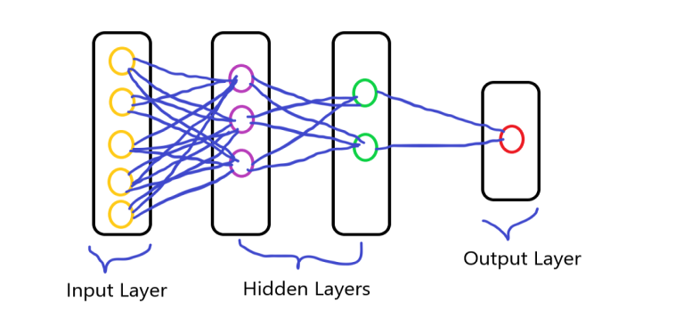
You all know that neurons are interconnected with each other in our brain and the process of transmitting data. It is similar to neurons in the human brain that are interconnected with each other, the neural network consists of a large number of artificial neurons, called units arranged in a sequence of layers. having the various layers of neurons and forming a complete network. these neurons are called nodes.
It consists of three layers which is:
- Input layerThe "input layer" refers to the initial level in a data analysis process or in neural network architectures. Its main function is to receive and process raw information before it is transformed by subsequent layers. In the context of machine learning, Proper configuration of the input layer is crucial to ensure the effectiveness of the model and optimize its performance in specific tasks....
- Hidden cloak
- Output layerThe "Output layer" is a concept used in the field of information technology and systems design. It refers to the last layer of a software model or architecture that is responsible for presenting the results to the end user. This layer is crucial for the user experience, since it allows direct interaction with the system and the visualization of processed data....
Create ANN Using a Breast Cancer Data Set
Now we move on to our topic, here we will take the dataset and then create the artificial neural network and classify the diagnosis, first, we take a breast cancer dataset and then move forward.
Data set: Breast Cancer Data Set
After downloading the dataset, we will import the important libraries that are required for further processing.
Import libraries
#import pandas
import pandas as pd
#import numpy
import numpy as np
import matplotlib.pyplot as plt
import seaborn as sb
Here we import pandas, NumPy and some display libraries.
Now we load our dataset using pandas:
df = pd.read_csv('Breast_cancer.csv')
df
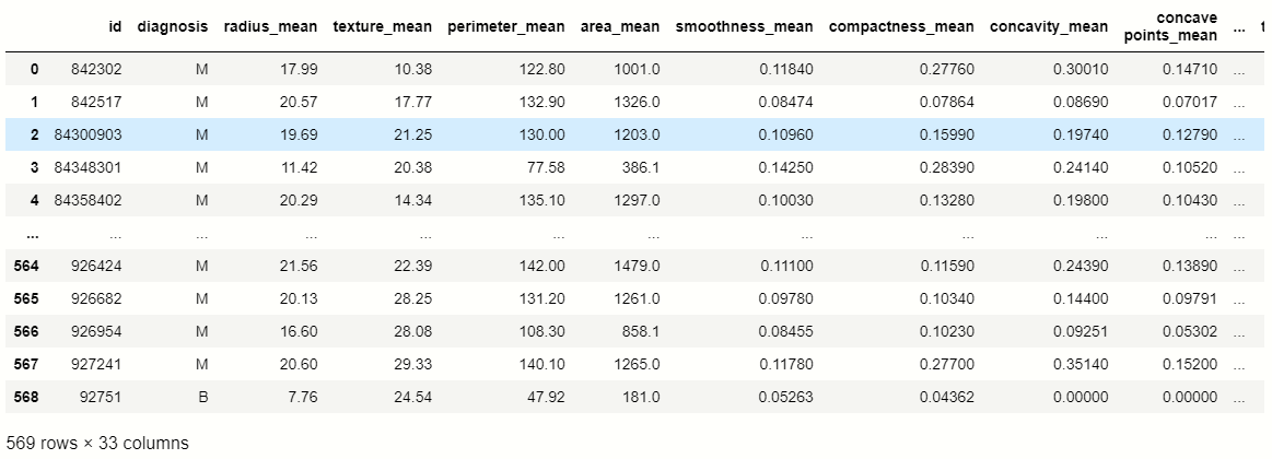
In this data set, we aim at the 'diagnosis’ characteristics column, so we check the count of values of that column using pandas:
# counting values of variables in 'diagnosis'
df['diagnosis'].value_counts()
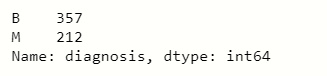
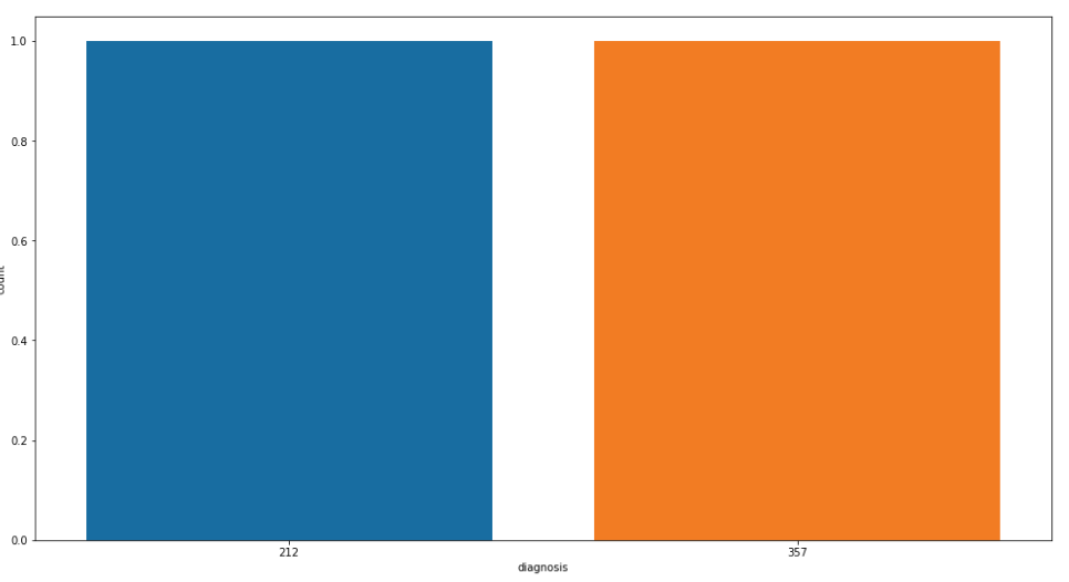
Now we visualize the counts of values of the ‘diagnostic columns: for better understanding
View value accounts
plt.figure(figsize=[17,9])
sb.countplot(df['diagnosis'].value_counts())
plt.show()
Null values
In the data set, we have to check the null values that are present inside the variables for which we use pandas:
df.isnull().sum()
After running the program, we conclude that the name of the function ‘Unnamed: 32’ contains all null values, so we delete or discard that column.
#droping feature
df.drop(['Unnamed: 32','id'],axis=1,inplace=True)
Independent and dependent variables
Now is the time to divide the data set into independent and dependent variables, for that we create two variables, one represents independent and the other represents dependent.
# independent variables
x = df.drop('diagnosis',axis=1)
#dependent variables
y = df.diagnosis
Management of categorical value
Cuando imprimimos la variableIn statistics and mathematics, a "variable" is a symbol that represents a value that can change or vary. There are different types of variables, and qualitative, that describe non-numerical characteristics, and quantitative, representing numerical quantities. Variables are fundamental in experiments and studies, since they allow the analysis of relationships and patterns between different elements, facilitating the understanding of complex phenomena.... dependent Y then we see that they contain categorical data and we have to convert categorical data to binary format for further processing. Therefore, we use Scikit learn Label Encoder to encode the categorical data.
from sklearn.preprocessing import LabelEncoder
#creating the object
lb = LabelEncoder()
y = lb.fit_transform(Y)
Data division
Ahora es el momento de dividir los datos en partes de trainingTraining is a systematic process designed to improve skills, physical knowledge or abilities. It is applied in various areas, like sport, Education and professional development. An effective training program includes goal planning, regular practice and evaluation of progress. Adaptation to individual needs and motivation are key factors in achieving successful and sustainable results in any discipline.... and test:
from sklearn.model_selection import train_test_split
xtrain,xtest,ytrain,ytest = train_test_split(x,Y,test_size=0.3,random_state=40)
Scale the data
When we created the artificial neural network, we have to scale the data to smaller numbers because the deep learning algorithm multiplies the weights and input data of the nodes and it takes a long time, so to reduce that time we scale the data.
to climb, we use scikit learn Standard climber module, we scale the training and test dataset:
#importing StandardScaler
from sklearn.preprocessing import StandardScaler
#creating object
sc = StandardScaler()
xtrain = sc.fit_transform(xtrain)
xtest = sc.transform(xtest)
From here we begin to create the artificial neural network, for that we import the important libraries that are used to create ANN:
#importing keras
import keras
#importing sequential module
from keras.models import Sequential
# import dense module for hidden layers
from keras.layers import Dense
#importing activation functions
from keras.layers import LeakyReLU,PReLU,ELU
from keras.layers import Dropout
Creating Layers
After importing those libraries, we create the three types of layers:
- Input layer
- Hidden cloak
- Output layer
First, we create the model:
#creating model
classifier = Sequential()
A sequential El modelo es apropiado para una pila simple de capas donde cada capa tiene exactamente un tensorTensors are mathematical structures that generalize concepts such as scalars and vectors. They are used in various disciplines, including physics, Engineering and Machine Learning, to represent multidimensional data. A tensor can be visualized as a multi-dimensional matrix, which allows complex relationships between different variables to be modeled. Their versatility and ability to handle large volumes of information make them fundamental tools in data analysis and processing.... de entrada y un tensor de salida.
Now we create the layers of the neural network:
#first hidden layer
classifier.add(Dense(units=9,kernel_initializer="he_uniform",activation='relu',input_dim=30))
#second hidden layer
classifier.add(Dense(units=9,kernel_initializer="he_uniform",activation='relu'))
# last layer or output layer
classifier.add(Dense(units=1,kernel_initializer="glorot_uniform",activation='sigmoid'))
In the following code, the Dense method is used to create the layers, en el que usamos parametersThe "parameters" are variables or criteria that are used to define, measure or evaluate a phenomenon or system. In various fields such as statistics, Computer Science and Scientific Research, Parameters are critical to establishing norms and standards that guide data analysis and interpretation. Their proper selection and handling are crucial to obtain accurate and relevant results in any study or project.... fundamentales. The first parameter is Exit nodes, the The second is the initializer for the kernel weights matrix, el tercero es la wake functionThe activation function is a key component in neural networks, since it determines the output of a neuron based on its input. Its main purpose is to introduce nonlinearities into the model, allowing you to learn complex patterns in data. There are various activation functions, like the sigmoid, ReLU and tanh, each with particular characteristics that affect the performance of the model in different applications.... y el último parámetro son los nodos de entrada o el número de características independientes.
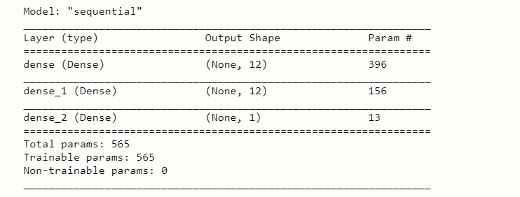
After executing this code we take the summary of it using:
#taking summary of layers
classifier.summary()
By filling in ANN
Now we compile our model with the optimizer:
#compiling the ANN
classifier.compile(optimizer="adam",loss="binary_crossentropy",metrics=['accuracy'])
Adaptation of the ANN to the training data
After compiling the model, we have to fit the ANN in the training data for the prediction:
 #fitting the ANN to the training set
model = classifier.fit(xtrain,ytrain,batch_size=100,epochs=100)
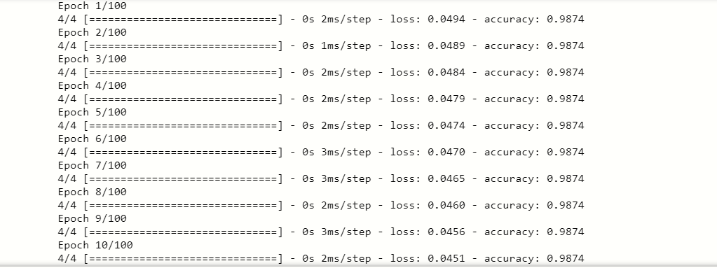
the to fit in() The method fits the ANN to the training data, in the parameters we set the specific values of each variable as lot size, epochs, etc. Finally, we found an excellent accuracy score, so our model is perfectly adapted to the training data.
After training the data, we also need to test the accuracy score of the test data, let's see next:
#now testing for Test data
y_pred = classifier.predict(test)
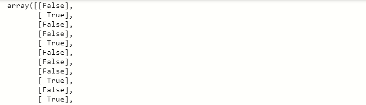
When running this code, we found that y_pred contained the different values, so we convert prediction values to threshold values as True, Fake.
#converting values
y_pred = (y_pred>0.5)
print(y_pred)
Punctuation and confusion matrix
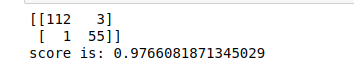
Now we check the confusion matrix and the score of the predicted values.
from sklearn.metrics import confusion_matrix
from sklearn.metrics import accuracy_score
cm = confusion_matrix(ytest,y_pred)
score = accuracy_score(ytest,y_pred)
print(cm)
print('score is:',score)
Production:-
Visualize confusion matrix
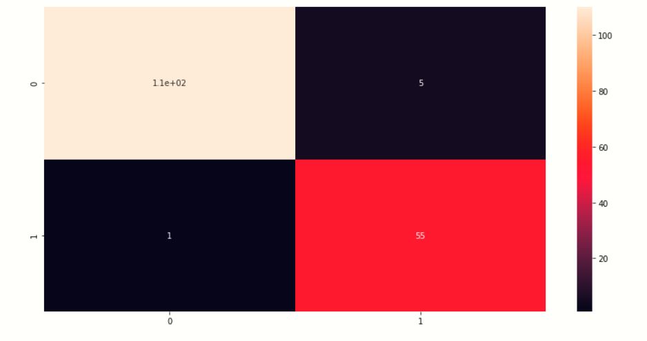
Here we visualize the confusion matrix of the prediction values.
# creating heatmap of comfussion matrix
plt.figure(figsize=[14,7])
sb.heatmap(cm,annot=True)
plt.show()
View data history
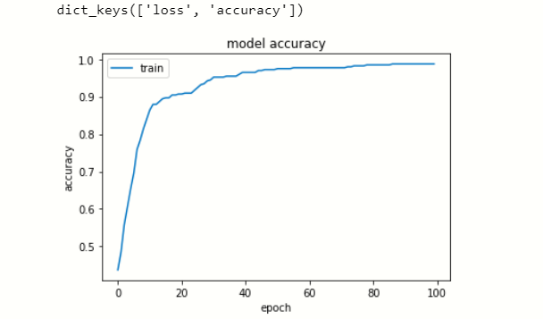
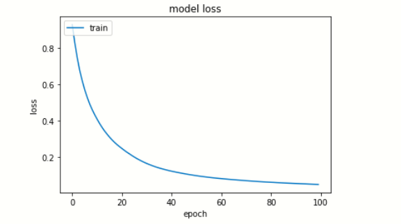
Now we visualize the loss and precision in each epoch.
# list all data in history
print(model.history.keys())
# summarize history for accuracy
plt.plot(model.history['accuracy'])
plt.title('model accuracy')
plt.ylabel('accuracy')
plt.xlabel('epoch')
plt.legend(['train', 'test'], loc ="upper left")
plt.show()
# summarize history for loss
plt.plot(model.history['loss'])
plt.title('model loss')
plt.ylabel('loss')
plt.xlabel('epoch')
plt.legend(['train', 'test'], loc ="upper left")
plt.show()
Savings model
Finally, we save our model.
#saving the model
classifier.save('File_name.h5')
EndNote
This is my first ANN created in deep learning, I am a beginner in deep learning. I do my best to explain this article, hope you like. Thanks for reading this article.
Connect with me on LinkedIn: Profile
Thanks.
The media shown in this article is not the property of DataPeaker and is used at the author's discretion.





