Detection and localization of brain tumors

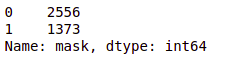
• Count the values ​​of each class.

brain_df['mask'].value_counts()

• Randomly display an MRI image from the dataset.

image = cv2.imread(brain_df.image_path[1301])
plt.imshow(image)

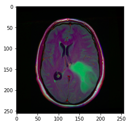
Image_path stores the path of the brain MRI so we can display the image using matplotlib.

Suggestion: the greenish part of the image above can be considered as the tumor.

• What's more, show the corresponding mask image.

image1 = cv2.imread(brain_df.mask_path[1301])
plt.imshow(image1)

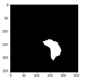
Now, you may have gotten the hint of what the mask really is. The mask is the image of the part of the brain affected by a tumor from the corresponding MRI image. Here, the mask is from the brain MRI shown above.

• Analyze the pixel values ​​of the mask image.

cv2.imread(brain_df.mask_path[1301]).max()

Departure: 255

The maximum value of pixels in the mask image is 255, what the white color indicates.

cv2.imread(brain_df.mask_path[1301]).min()

Departure: 0

The minimum value of pixels in the mask image is 0, what the black color indicates.

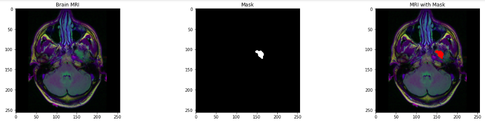
• Visualization of MRI of the brain, the corresponding mask and MRI with the mask.

count = 0
fig, axs = plt.subplots(12, 3, figsize = (20, 50))
for i in range(len(brain_df)):
  if brain_df['mask'][i] ==1 and count <5:
    img = io.imread(brain_df.image_path[i])
    axs[count][0].title.set_text('Brain MRI')
    axs[count][0].imshow(img)
    
    mask = io.imread(brain_df.mask_path[i])
    axs[count][1].title.set_text('Mask')
    axs[count][1].imshow(mask, cmap = 'gray')
    
    img[mask == 255] = (255, 0, 0) #Red color
    axs[count][2].title.set_text('MRI with Mask')
    axs[count][2].imshow(img)
    count+=1

fig.tight_layout()

• Remove identification, as it is not necessary for processing.

# Drop the patient id column
brain_df_train = brain_df.drop(columns = ['patient_id'])
brain_df_train.shape

You will get the size of the data frame in the output: (3929, 3)

• Convert data in mask column from integer format to string format, since we will need the data in string format.

brain_df_train['mask'] = brain_df_train['mask'].apply(lambda x: str(x))
brain_df_train.info()

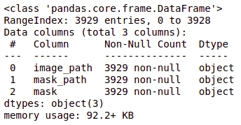
As you can see, now each feature has data type as object.

• Divide the data into test and train sets.

# split the data into train and test data from sklearn.model_selection import train_test_split train, test = train_test_split(brain_df_train, test_size = 0.15)

• Increase more data with ImageDataGenerator. ImageDataGenerator generates batches of tensioner image data with real-time data augmentation.

Refer here for more information about ImageDataGenerator and parameters in detail.

We will create a train_generator and validation_generator from the train data and a test_generator from the test data.

# create an image generator
from keras_preprocessing.image import ImageDataGenerator

#Create a data generator which scales the data from 0 to 1 and makes validation split of 0.15
datagen = ImageDataGenerator(rescale=1./255., validation_split = 0.15)

train_generator=datagen.flow_from_dataframe(
dataframe=train,
directory= './',
x_col="image_path",
y_col ="mask",
subset="training",
batch_size=16,
shuffle=True,
class_mode="categorical",
target_size=(256,256))

valid_generator=datagen.flow_from_dataframe(
dataframe=train,
directory= './',
x_col="image_path",
y_col ="mask",
subset="validation",
batch_size=16,
shuffle=True,
class_mode="categorical",
target_size=(256,256))

# Create a data generator for test images
test_datagen=ImageDataGenerator(rescale=1./255.)

test_generator=test_datagen.flow_from_dataframe(
dataframe=test,
directory= './',
x_col="image_path",
y_col ="mask",
batch_size=16,
shuffle=False,
class_mode="categorical",
target_size=(256,256))