Difference between R-squared and adjusted R-squared

Overview

• Understand the concept of R squared and adjusted R squared
• Learn the key differences between R-squared and adjusted R-squared

Introduction

When I started my journey in data science, the first algorithm I explored was linear regression. After understanding the concepts of linear regression and how the algorithm works, I was really excited to use it and make predictions on a problem statement. I'm sure most of you would have done the same. But once we have predicted the values, Whats Next?

Then comes the tricky part. Once we have built our model, the next step was to evaluate their performance. It goes without saying that the task of evaluating the model is critical and highlights the shortcomings of our model.. Choose the most suitable Evaluation metric it is a crucial task. And I found two important metrics: R-squared and R-squared adjusted apart from MAE / MSE / RMSE. What is the difference between these two? Which one should I use?

R squared and adjusted R squared are two of these evaluation metrics that may seem confusing to any aspiring data science initially.. Since both are extremely important for evaluating regression problems, we are going to understand and compare them in depth. Both have their pros and cons, which we will discuss in detail in this article.

Note: To understand R-squared and adjusted R-squared, must have a good knowledge of linear regression. Check out our free course –

Table of Contents

• Residual sum of squares
• Understanding the R-squared statistic
• Problems with the R-squared statistic
• Adjusted R-squared statistic

Residual sum of squares

To understand the concepts clearly, we will tackle a simple regression problem. Here, we are trying to predict the ‘grades obtained’ depending on the amount of 'time spent studying'. the weather spent studying will be ours independent variable and the trademarks accomplished in the test is ours dependent O target variable.

We can plot a simple regression graph to visualize this data.

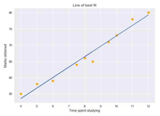
The yellow points represent the data points and the blue line is our predicted regression line. As you can see, our regression model does not perfectly predict all data points. Then, How do we evaluate the predictions of the regression line using the data? Good, we could start by determining the residual values ​​for the data points.

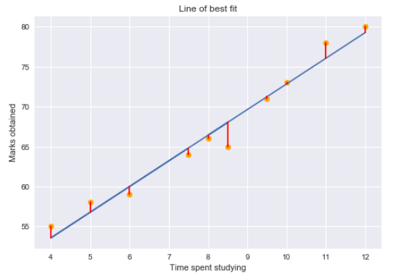
Residual for a point in the data is the difference between the actual value and the value predicted by our linear regression model.

Residual plots tell us if the regression model is right for the data or not. In reality, it is an assumption of the regression model that there is no trend in the residual plots. To study the assumptions of linear regression in detail, I suggest going through this great artitle!

Using residual values, we can determine the sum of the squares of the residuals also known as Residual sum of squares or RSS.

The lower the RSS value, the better the model predictions. Or we can say that a regression line is a line of best fit if you minimize the value of RSS. But there is a flaw in this: RSS is a scale variant statistic. Since RSS is the sum of the squared difference between the actual and predicted value, the value depends on the scale of the target variable.

Example:

Consider that your target variable is the income generated from the sale of a product. The residuals would depend on the scale of this objective. If the income scale is taken in “Hundreds of rupees” (namely, the goal would be 1, 2, 3, etc.), then we could get an RSS of about 0,54 (speaking hypothetically).

But if the target income variable was taken in “rupees” (namely, the goal would be 100, 200, 300, etc.), then we could get a higher RSS like 5400. Although the data does not change, the value of RSS varies. according to the target scale. This makes it difficult to judge what might be a good RSS value..

Then, Can we come up with a better statistic that is scale invariant? This is where R-square comes into the picture..

Understanding the R-squared statistic

The R-squared statistic or coefficient of determination is a scale invariant statistic that provides the proportion of variation in the target variable explained by the linear regression model..

This may seem a bit complicated, so let me break it down here. To determine the proportion of target variation explained by the model, we must first determine the following:

1. Total sum of squares

   The total variation of the target variable is the sum of the squares of the difference between the real values ​​and their mean.

   

   TSS or total sum of squares gives the total variation in Y. We can see that it is very similar to the variance of Y. While the variance is the average of the squared sums of difference between the real values ​​and the data points, TSS is the total of the squared sums.

   Now that we know the total variation in the target variable, How do we determine the proportion of this variation explained by our model? We return to RSS.

2. Residual sum of squares

   As we commented before, RSS gives us the total square of the distance of the real points from the regression line. But if we focus on a single residue, we can say that it is the distance that is not captured by the regression line. Therefore, RSS as a whole gives us the variation in the target variable which is not explained by our model.

3. Calculate R-squared

Now, if TSS gives us the total variation in Y, and RSS gives us the variation in Y not explained by X, then TSS-RSS gives us the variation in Y that is explained by our model! We can simply divide this value by TSS to obtain the proportion of variation in Y that the model explains. And this ours R-squared statistic!

R-square = (TSS-RSS) / TSS

= Variation explained / Total variation

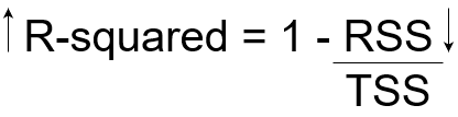
= 1 – Unexplained variation / Total variation

Then, R squared gives the degree of variability in the target variable that is explained by the model or the independent variables. If this value is 0,7, means that the independent variables explain the 70% of the variation in the target variable.

The value of R squared is always between 0 Y 1. A higher R squared value indicates a greater amount of variability explained by our model and vice versa..

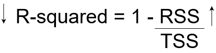
If we had a really low RSS value, it would mean that the regression line was very close to the real points. This means that the independent variables explain most of the variation in the target variable.. In that case, we would have a really high R-squared value.

Conversely, if we had a really high RSS value, it would mean that the regression line would be very far from the real points. Therefore, the independent variables fail to explain most of the variation in the target variable. This would give us a really low R-squared value.

Then, this explains why the R-squared value gives us the variation in the target variable given by the variation in the independent variables.

Problems with the R-squared statistic

The R squared statistic is not perfect. In fact, suffers from a major defect. Its value never decreases no matter how many variables we add to our regression model. Namely, even if we add redundant variables to the data, the value of R squared does not decrease. Either stays the same or increases with the addition of new independent variables. This clearly does not make sense because some of the independent variables may not be useful in determining the target variable.. Adjusted R-square takes care of this problem.

Adjusted R-squared statistic

The adjusted R-squared takes into account the number of independent variables used to predict the target variable.. In doing so, we can determine whether adding new variables to the model actually increases the fit of the model.

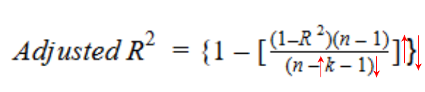
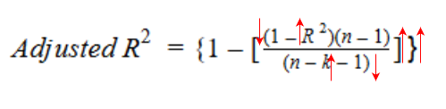
Let's take a look at the adjusted R-squared formula to better understand how it works..

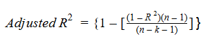
Here,

• North represents the number of data points in our data set
• k represents the number of independent variables, Y
• R represents the R squared values ​​determined by the model.

Then, if R-squared does not increase significantly with the addition of a new independent variable, then the adjusted R-squared value will actually decrease.

Secondly, if when adding the new independent variable we see a significant increase in the value of R squared, then the adjusted R squared value will also increase.

We can see the difference between the R squared and adjusted R squared values ​​if we add a random independent variable to our model.

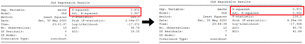
As you can see, adding a random independent variable did not help explain the variation in the target variable. Our R squared value remains the same. Therefore, gives us a false indication that this variable could be useful in predicting the output. But nevertheless, the adjusted R-squared value decreased, which indicated that this new variable is not actually capturing the trend in the target variable.

Clearly, it is better to use adjusted R-squared when there are multiple variables in the regression model. This would allow us to compare models with different numbers of independent variables.

Final notes

In this article, we analyze what the R-squared statistic is and where it fails. We also take a look at adjusted R squared.

Hopefully, this has given him a better understanding of things. Now you can wisely determine which independent variables are useful in predicting the outcome of your regression problem..

To learn more about other evaluation metrics, I suggest checking out the following great resources:

Related