In my previous article, “Combining data sets in SAS – Simplified”, we analyze three methods for combining data sets: attach, concatenate and merge. In this article, we will see the most common and used method to combine data sets: MERGER or UNION.
The need to unite / merge data sets:
Before going into details, let's understand why we really need to come together / merge. Whenever we have information divided and available in two or more data sets and we want to combine them in a single data set, we need to merge / join these tables. One of the main things to keep in mind is that the merge should be based on common criteria or fields. For instance, in a retail company, we have a table of daily transactions (table contains product details, sales details and customer details) and an inventory table (which has product details and available quantity). However, to have the information about Inventory or the availability of a product, what should we do? Combine the table TransactionThe "transaction" refers to the process by which an exchange of goods takes place, services or money between two or more parties. This concept is fundamental in the economic and legal field, since it involves mutual agreement and consideration of specific terms. Transactions can be formal, as contracts, or informal, and are essential for the functioning of markets and businesses.... with the Product_Code-based inventory table, and subtract the quantity sold from the quantity on hand.
The fusion / union can be of various types and depends on business requirements and relationship between data sets. First, Let's look at various types of relationships that data sets can have.
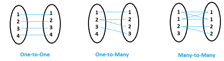
- When for each value of variableIn statistics and mathematics, a "variable" is a symbol that represents a value that can change or vary. There are different types of variables, and qualitative, that describe non-numerical characteristics, and quantitative, representing numerical quantities. Variables are fundamental in experiments and studies, since they allow the analysis of relationships and patterns between different elements, facilitating the understanding of complex phenomena.... common (let's say Variable 'x') in the first data set, the second data set has only one matching value for that common variable 'x', then it's called Twelve fifty-nine relationship.
- When for the values of the common variable (let's say variable 'y') in the first data set, other data sets have more than one matching value for that common variable 'y', then it's called One to many relationship.
- When both data sets have multiple entries for the same common variable value, then it's called Many to many relationship.
And SAS, we can make unions / mergers through various forms, here we will discuss the most common ways: Data Step y PROC SQL. In the Data step, we use the Merge instruction to perform joins, while in PROC SQL, we write a SQL query. Let's analyze the data pass first:
DATA STEPS
Syntax:-
 Data Dataset;
 Merge Dataset1 Dataset2 Dataset3 ...Datasetn;
 By CommonVariable1 CommonVariable2......CommonVariablen;
 Run;
Note: – Data sets must be sorted by variable (s) common and name, common variable type and length must be the same for all input data sets.
Let's look at some scenarios for each of the relationships between input data sets.
ONE to ONE relationship
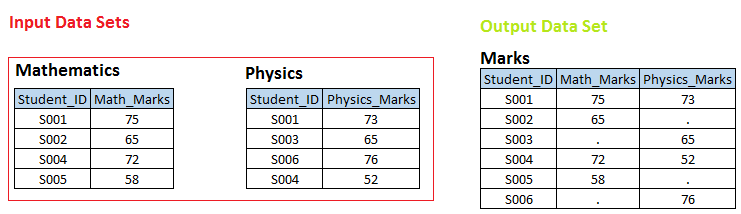
Stage 1 In the following input data sets, you can see that there is a one-to-one relationship between these two tables in Student ID. Now we want to create a dataset. BRANDS, where we have all the unique student_ids with the respective math and physics grades. If student_id is not available in Math table, so math_marks should have a missing value and vice versa.
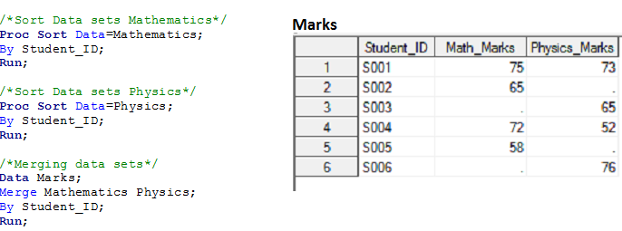
Solution using Data Steps: –
How does it work:-
- SAS compares both data sets and creates a POS (Program data vector) for all unique variables and initializes them with missing values (the Program Data Vector is an intermediary between the input and output data sets). In the current example, I would create a POV like this:

- Read the first observation from the input data sets and compare the values of the BY variable in both data sets:
- if the values are equal, it is compared with the value of the BY variable in POS.
- if not the same, the POV variables are reset with the missing values and the current observation value is copied to the POV while the other observation remains lost
- If it's the same, POS variables are not reinitialized. The available value of the current observation is updated in the POS
- Thereafter, the record pointer moves to the next observation in both data sets and, while the RUN instruction is executing, PDV values are passed to the output data set.
- If the value of By variable does not match, the observation of the data set with the lowest value is copied to POS. The record pointer of the dataset that has a lower BY variable value is moved to the next observation and step 2 (a) repeats again.
- if the values are equal, it is compared with the value of the BY variable in POS.
- The above steps are repeated until the EOF of both data sets is reached.
You can run a trial to evaluate the result data set.
Stage 2: – Based on the input data sets of the scenario 1, we want to create the following output data sets.
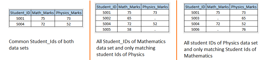
Solution using data steps: – Let's write a code similar to the scenario 1 with the IN option. 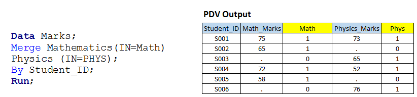 Above, you can see that we have used the IN option with both input data sets and assigned values of these to the temporary variables MATH and PHYS because they are temporary variables, so we can't see them in the output dataset.
I have shown you the table (PDV data) which has a variable value for all observations along with the temporary variables. Now, based on the value of these variables, we can write code for subconfiguration operations and JOIN"JOIN" is a fundamental operation in databases that allows you to combine records from two or more tables based on a logical relationship between them. There are different types of JOIN, as INNER JOIN, LEFT JOIN and RIGHT JOIN, each with its own characteristics and uses. This technique is essential for complex queries and more relevant and detailed information from multiple data sources.... as we need:
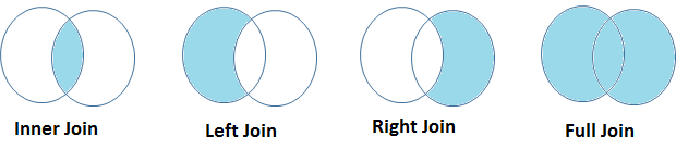
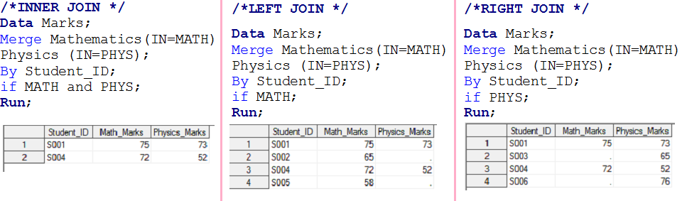
- If MATH and PHYS have value 1, will create the first output dataset and will be called INNER JOINa "Inner Join" is an operation in databases that allows you to combine rows of two or more tables, based on a specific match condition. This type of join only returns rows that have correspondences in both tables, resulting in a result set that reflects only the related data. It is critical in SQL queries to obtain cohesive and accurate information from multiple data sources.....
- If MATH has 1, will create a second set of output data and will be called LEFT JOINThe "LEFT JOIN" is an operation in SQL that allows you to combine rows from two tables, Showing all rows in the left table and matches in the right table. If there are no matches, are filled with null values. This tool is useful for getting complete information, Even when some relationships are optional, thus facilitating data analysis in an efficient and consistent manner.....
- If PHYS has 1, will create a third set of output data and will be called as RIGHT JOINThe "RIGHT JOIN" is an operation in databases that allows you to combine rows from two tables, ensuring that all rows in the table on the right are included in the result, even if there are no matches in the table on the left. This type of join is useful for preserving information from the secondary table, making it easy to analyze and obtain complete data in SQL queries....
- If MATH and PHYS have 1, will function as FULL JOINThe "FULL JOIN" is a database operation that combines the results of two tables, showing all records for both. When there are coincidences, data is combined, but records that do not have a correspondence in the other table are also included, completing with null values. This technique is useful for getting a complete view of the information, allowing a more exhaustive analysis of the data in relation to...., has also been resolved on stage-1.
ONE to MANY relationship
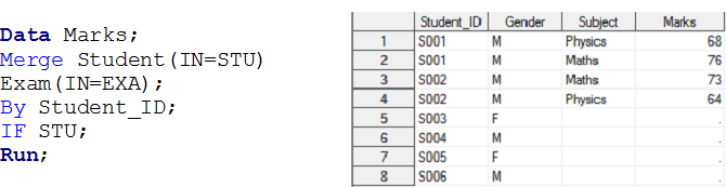
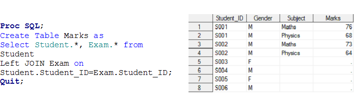
Stage – 3 Here we have two data sets, Student Y Exam and we want to create a set of output data Trademarks.
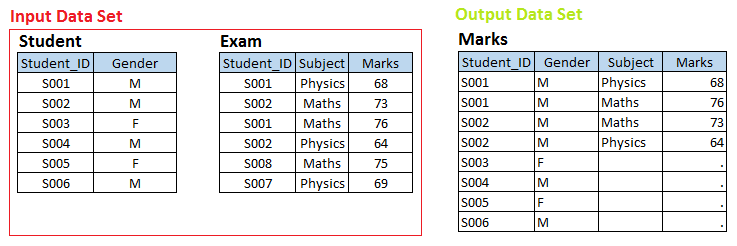
On top of input data sets, there is a one-to-many relationship between the student and the exam. Now, if you want to create output data set marks with individual observation for each student exam, these belong to the STUDENT data set, namely, Union left.
Solution using Data Steps: –
Similarly, we can perform operations for inner join, right and full for a one-to-many relationship using the IN operator.
MANY to MANY ratio
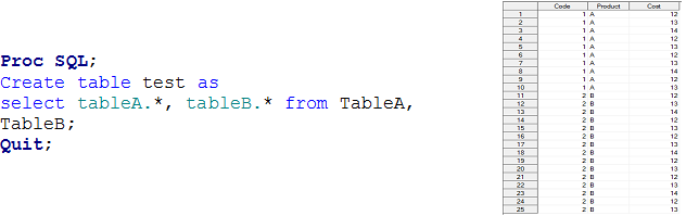
Stage 4: Create output data sets that have all joins based on a common field. You can also see that both input data sets have a many-to-many relationship.
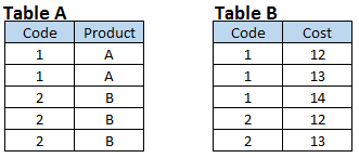
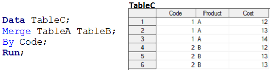
Data steps do not make a MANY to MANY relationship, because they do not provide output as a Cartesian product. When we merge table A and table B using data steps, the output is similar to the following snapshot.
 We have previously seen, How can we use data steps to merge two or more data sets that have any of the relationships, except MANY to MANY? Now we will see the PROC SQL methods to have a solution for similar requirements.
PROC SQL
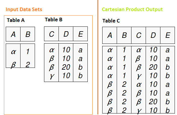
To understand join methodology in SQL, we must first understand the Cartesian product. The Cartesian product is a query that has multiple tables in the from clause and produces all possible combinations of rows from the input tables. If we have two tables with 2 Y 4 records respectively, using the cartesian product, we have a table with 2 X 4 = 8 records.
SQL joins work for each of the relationships between data sets (one by one, one to many and many to many). Let's see how it works with types of joins.
Syntax:-
Please select Column-1, Column-2,… Column-n of table1 INTERIOR JOINT / LEFT / RIGHT / COMPLETE tcapaz2 UPON Join-condition ;
Note:-
- Tables may or may not be ordered by common variables.
- The name of the common variables may not be similar, but it must be similar in length and type.
- Works with a maximum of two tables.
Let's solve the above requirements using PROC SQL.
Stage 1 :- This was an example of FULL Join, where all Student_IDs were required in the output dataset with the respective MATH and PHYSICS flags.
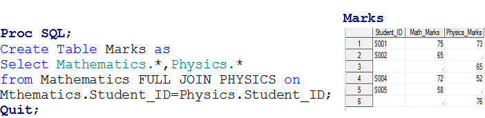
Up in the output data set, you can see that Student_ID is missing for those students who showed up for Physics exam only. To solve it we will use a COALESCE function. Returns the value of the first argument that is not missing from the given variables.
Syntax:-
COALESCE (argument-1, argument-2,… ..argument-n)
Let's modify the above code: –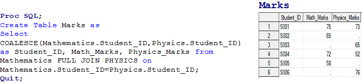
Stage 2: – This was an example of INNER, Left y Right Join. Here we are solving for Inner Join.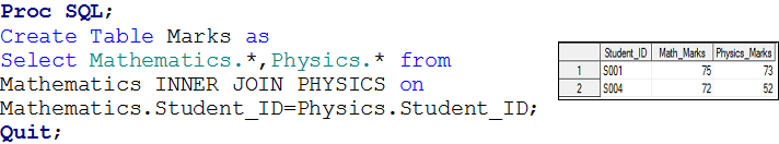 In the same way, we can do for left and right junction.
Stage -3 This was a left join issue for a ONE to MANY relationship.
Stage -4 This was a Many to MANY relationship issue.. We have already discussed that SQL can produce a Cartesian product that contains all record combinations between two tables.
Above we have seen Proc SQL to join / merge data sets.
Final note: –
In this series of articles on combining data sets in SAS, we analyze various methods to combine data sets such as adding, concatenar, merge, fuse. Particularly in this article, we discuss that depending on the relationship between data sets, various types of joins and how we can solve it based on different scenarios. We have used two methods (Data Steps y PROC SQL) to achieve results. We will see the efficiency of these methods in one of the future articles..
Has this series been useful to you? We have simplified a complex topic like combining data sets and tried to present it in an understandable way. If you need more help with combining data sets, feel free to ask your questions through the comments below.
PS Have you joined? Analytical Vidhya Discuss yet? If that is not the case, a lot of data science debates are being lost. These are some of the discussions that take place in SAS:
1. Select variables and transfer them to a new dataset in SAS
2. Import the first 20 records from Excel to SAS
3. Where the statement does not work in SAS


