This article was published as part of the Data Science Blogathon
Imputation is a technique used to replace missing data with some surrogate value to retain most of the data / dataset information. These techniques are used because removing the data from the dataset each time is not feasible and can lead to a reduction in the size of the dataset to a great extent., which not only raises concerns about skewing the data set, it also leads to incorrect analysis.
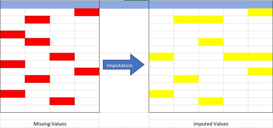
Source: created by the author
Not sure what data is missing? How does it happen? And your type? Take a look HERE to learn more about it.
Let's understand the concept of imputation from Fig {Fig 1} anterior. In the picture above, I have tried to represent the missing data in the table on the left (marked in red) and by using imputation techniques we have completed the missing data set in the table on the right (marked in yellow), without reducing the actual size of the dataset. If we realize here, we have increased the size of the column, what is possible in the imputation (adding the category imputation “Lack”).
Why is imputation important?
Then, after knowing the definition of imputation, the next question is why should we use it and what would happen if I don't use it?
Here we go with the answers to the previous questions.
We use imputation because missing data can cause the following problems: –
- Incompatible with most Python libraries used in Machine Learning: – Yes, you read well. When using the libraries for ML (the most common is skLearn), do not have a provision to automatically handle this missing data and can generate errors.
- Distortion in the data set: – A large amount of missing data can cause distortions in the distribution of the variable, namely, can increase or decrease the value of a particular category in the data set.
- Affects the final model: – missing data can cause bias in the dataset and can lead to faulty analysis by the model.
Another and the most important reason is “We want to restore the complete dataset”. This occurs mainly in the case where we do not want to lose (plus) data from our dataset, since all are important and, Secondly, the size of the dataset is not very large and removing part of it can have a significant impact. in the final model.
Excellent..!! we got some basics of missing data and imputation. Now, Let's take a look at the different imputation techniques and compare them. But before jumping into it, we have to know the data types in our dataset.
It sounds strange..!!! Don't worry ... Most of the data is from 4 types: – Numeric, Categorical, Date-time and Mixed. These names are self explanatory, so they do not delve much or describe them.
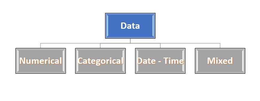
Fig 2: – Type of data
Source: created by the author
Imputation techniques
Moving on to the highlights of this article … Techniques used in imputation …
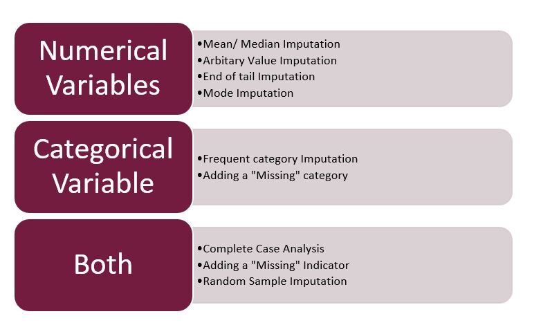
Fig 3: – Imputation techniques
Source: created by the author
Note: – Here I will focus solely on the mixed imputation, numerical and categorical. The date and time will be part of the next article.
1. Full case analysis (CCA): –
This is a fairly straightforward method to handle missing data, which directly removes the rows that have missing data, namely, we consider only those rows in which we have complete data, namely, no missing data. This method is also popularly known as “delete by list”.
- Assumptions: –
- Random data is missing (MAR).
- Missing data is completely removed from the table.
- Advantage: –
- Easy to implement.
- No data manipulation required.
- Limitations: –
- Deleted data may be informative.
- It can lead to the deletion of much of the data.
- You can create a bias in the dataset, if a large amount of a particular type of variable is removed.
- The production model will not know what to do with the missing data.
- When to use:-
- The data is MAR (Missing At Random).
- Good for mixed data, numerical and categorical.
- The missing data is no more than 5% to 6% of the data set.
- The data does not contain much information and will not skew the data set.
- Code:-
## To check the shape of original dataset
train_df.shape
## Output (614 rows & 13 columns)
(614,13)
## Finding the columns that have Null Values(Missing Data)
## We are using a for loop for all the columns present in dataset with average null values greater than 0
na_variables = [ var for var in train_df.columns if train_df[where].isnull().mean() > 0 ]
## Output of column names with null values
['Gender','Married','Dependents','Self_Employed','LoanAmount','Loan_Amount_Term','Credit_History']
## We can also see the mean null values present in these columns {Shown in the image below}
data_na = trainf_df[na_variables].isnull (). mean ()
## Implementing the CCA techniques to remove Missing Data
data_cca = train_df(axis=0)  ### axis=0 is used for specifying rows
## Verifying the final shape of the remaining dataset
data_cca.shape
## Output (480 rows & 13 Columns)
(480,13)
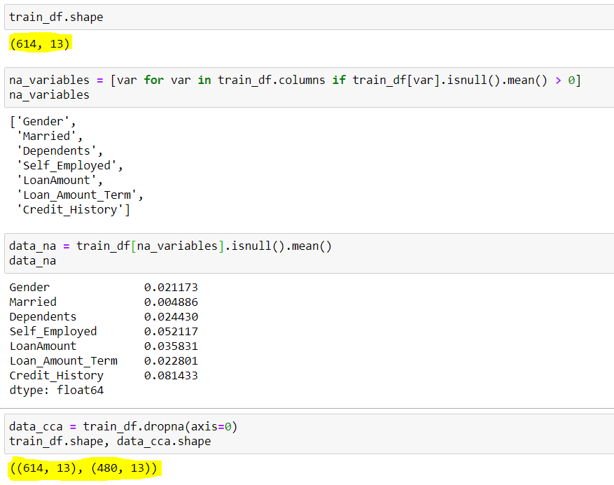
Figure 3: – CCA
Source: Created by the author
Here we can see, the dataset initially had 614 rows and 13 columns, of which 7 rows had missing data(variables_variables), its missing middle rows are shown by data_na. We observed that, apart from and , all have an average lower than 5%. Then, according to CCA, we remove the rows with missing data, which resulted in a data set with only 480 rows. Here you can see around the 20% of data reduction, which can cause a lot of problems in the future.
2. Arbitrary Value Imputation
This is an important technique used in imputation, since it can handle both numeric and categorical variables. This technique states that we group the missing values in a column and assign them to a new value that is far from the range of that column. In general, we use values like 99999999 O -9999999 O “Lack” O “Undefined” for numerical and categorical variables.
- Assumptions: –
- Data is not lacking at random.
- Missing data is imputed with an arbitrary value that is not part of the data set or the mean / median / data fashion.
- Advantage: –
- Easy to implement.
- We can use it in production.
- Preserves the importance of “missing values” if it exists.
- Disadvantages: –
- You can distort the distribution of the original variable.
- Arbitrary values can create outliers.
- Extra caution is required when selecting the arbitrary value.
- When to use:-
- When the data is not MAR (Missing At Random).
- fit for all.
- Code:-
## Finding the columns that have Null Values(Missing Data)
## We are using a for loop for all the columns present in dataset with average null values greater than 0
na_variables = [ var for var in train_df.columns if train_df[where].isnull().mean() > 0 ]
## Output of column names with null values
['Gender','Married','Dependents','Self_Employed','LoanAmount','Loan_Amount_Term','Credit_History']
## Use Gender column to find the unique values in the column
train_df['Gender'].unique()
## Output
array(['Male','Female',in])
## Here nan represent Missing Data
## Using Arbitary Imputation technique, we will Impute missing Gender with "Missing"  {You can use any other value also}
arb_impute = train_df['Gender'].fillna('Missing')
unique impute.arb()
## Output
array(['Male','Female','Missing'])
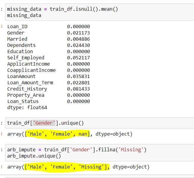
Fig 4: – Arbitrary imputation
Source: created by the author
We can see here the column Gender I had 2 unique values {‘Male female’} and few missing values {in}. When using arbitrary imputation, we fill the values of {in} in this column with {missing}, for what you get 3 unique values for the variable ‘Gender’.
3. Frequent category imputation
This technique says to replace the missing value with the variable with the highest frequency or in simple words by replacing the values with the Mode of that column. This technique is also known as Mode imputation.
- Assumptions: –
- Random data is missing.
- There is a high probability that the missing data will look like most of the data.
- Advantage: –
- Implementation is simple.
- We can get a complete data set in a very short time.
- We can use this technique in the production model.
- Disadvantages: –
- The higher the percentage of missing values, the greater the distortion.
- May lead to overrepresentation of a particular category.
- You can distort the distribution of the original variable.
- When to use:-
- Random data is missing (MAR)
- The missing data is no more than 5% to 6% of the data set.
- Code:-
## finding the count of unique values in Gender
train_df['Gender'].groupby(train_df['Gender']).count()
## Output (489 Male & 112 Female)
Male 489
Female 112
## Male has higgest frequency. We can also do it by checking the mode
train_df['Gender'].mode()
## Output
Male
## Using Frequent Category Imputer
frq_impute = train_df['Gender'].fillna('Male')
frq_impute.unique()
## Output
array(['Male','Female'])
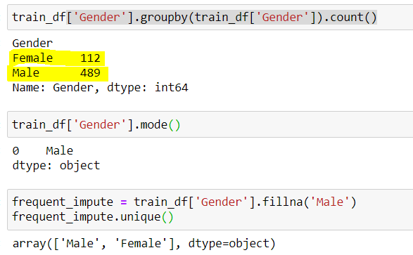
Fig 4: – Frequent category imputation
Source: created by the author
Here we note that “Masculine” was the most frequent category, so we use it to replace the missing data. Now we are left alone 2 categories, namely, male and female.
Therefore, we can see that each technique has its advantages and disadvantages, and it depends on the data set and the situation for which the different techniques that we are going to use.
That's all from here …
Until then, este es Shashank Singhal, a Big Data and data science enthusiast.
Happy learning ...
If you liked my article you can follow me HERE
Linkedin profile:- www.linkedin.com/in/shashank-singhal-1806
Note: – All images used above were created by me (Author).
The media shown in this article is not the property of DataPeaker and is used at the author's discretion.


