Machine learning with Python: Logistic regression

What is logistic regression?

This article assumes that you have a basic knowledge and understanding of machine learning concepts., as the target vector, the matrix of characteristics and related terms.

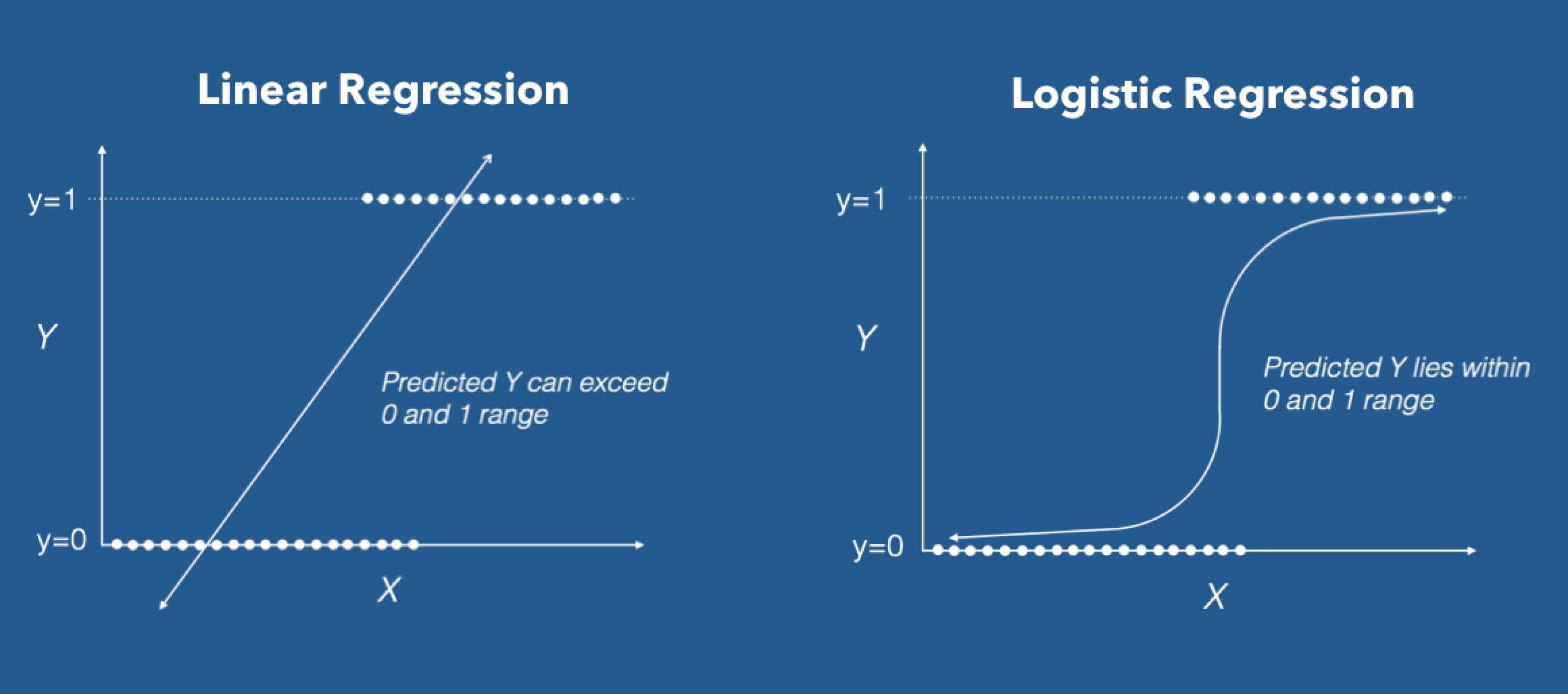
Logistic regression: probably one of the most interesting supervised machine learning algorithms in machine learning. Despite having “Regression” in her name, Logistic regression is a popularly used supervised method. Classification Algorithm. Logistic regression, along with their related cousins ​​viz.. Multinomial logistic regression, gives us the ability to predict whether an observation belongs to a certain class using an approach that is simple, easy to understand and on.

Source: DZone

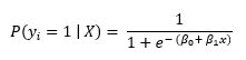
Logistic regression in its base form (by default) it's a Binary classifier. This means that the target vector can only take the form of one of two values. In the formula of the logistic regression algorithm, we have a linear model, for instance, b₀ + b₁x, which is integrated into a logistics function (also known as sigmoid function). The formula of the Binary Classifier that we have at the end is the following:

Where:

• P (Y_I = 1 | X) is the probability of the i^th Observations target value, Y_I belonging to the class 1.
• Β₀ y β₁ are the parameters to be learned.
• me represents Euler's number.

Main objective of the logistic regression formula.

The logistic regression formula aims to limit or constrain the linear output and / the sigmoid between a value of 0 Y 1. The main reason is for interpretability purposes, namely, we can read the value as a simple probability; Which means that if the value is greater than 0,5, class one would be predicted; on the contrary, class is predicted 0.

Source: GraphPad

Python implementation.

Now we will see the implementation of the Python programming language. For this exercise, We will use the ionosphere dataset that is available for download from the UCI machine learning repository.

# We begin by importing the necessary packages
# to be used for the Machine Learning problem

import pandas as pd
import numpy as np
from sklearn.linear_model import LogisticRegression
from sklearn.preprocessing import StandardScaler

# We read the data into our system using Pandas'
# 'read_csv' method. This transforms the .csv file
# into a Pandas DataFrame object.

dataframe = pd.read_csv('ionosphere.data', header=None)

# We configure the display settings of the
# Pandas DataFrame.

pd.set_option('display.max_rows', 10000000000)
pd.set_option('display.max_columns', 10000000000)
pd.set_option('display.width', 95)

# We view the shape of the dataframe. Specifically
# the number of rows and columns present.
print('This DataFrame Has %d Rows and %d Columns'%(dataframe.shape))

The output to the previous code would be the following (the shape of the data frame):

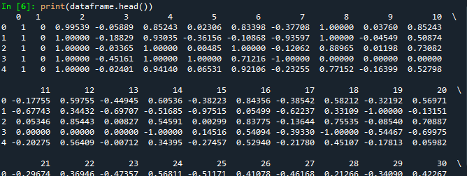
# We print the first five rows of our dataframe.
print(dataframe.head())

The output of the above code will look like the following (the following output is truncated):

# We isolate the features matrix from the DataFrame.
features_matrix = dataframe.iloc[:, 0:34]

# We isolate the target vector from the DataFrame.
target_vector = dataframe.iloc[:, -1]

# We check the shape of the features matrix, and target vector.
print('The Features Matrix Has %d Rows And %d Column(s)'%(features_matrix.shape))
print('The Target Matrix Has %d Rows And %d Column(s)'%(np.array(target_vector).reshape(-1, 1).shape))

The output for the shape of our feature matrix and the target vector would be the following:

# We use scikit-learn's StandardScaler in order to
# preprocess the features matrix data. This will
# ensure that all values being inputted are on the same
# scale for the algorithm.

features_matrix_standardized = StandardScaler().fit_transform(features_matrix)

# We create an instance of the LogisticRegression Algorithm
# We utilize the default values for the parameters and
# hyperparameters.

algorithm = LogisticRegression(penalty='l2', dual=False, toll=1e-4,
C=1.0, fit_intercept=True,
intercept_scaling=1, class_weight=None,
random_state=None, solver="lbfgs",
max_iter=100, multi_class="auto",
verbose=0, warm_start=False, n_jobs=None,
l1_ratio=None)

# We utilize the 'fit' method in order to conduct the
# training process on our features matrix and target vector.

Logistic_Regression_Model = algorithm.fit(features_matrix_standardized, target_vector)

# We create an observation with values, in order
# to test the predictive power of our model.

observation = [[1, 0, 0.99539, -0.05889, 0.8524299999999999, 0.02306,
0.8339799999999999, -0.37708, 1.0, 0.0376,
0.8524299999999999, -0.17755, 0.59755, -0.44945, 0.60536,
-0.38223, 0.8435600000000001, -0.38542, 0.58212, -0.32192,
0.56971, -0.29674, 0.36946, -0.47357, 0.56811, -0.51171,
0.41078000000000003, -0.46168000000000003, 0.21266, -0.3409,
0.42267, -0.54487, 0.18641, -0.453]]

# We store the predicted class value in a variable
# called 'predictions'.

predictions = Logistic_Regression_Model.predict(observation)

# We print the model's predicted class for the observation.
print('The Model Predicted The Observation To Belong To Class %s'%(predictions))

The output to the previous code block should be as follows:

# We view the specific classes the model was trained to predict.

print('The Algorithm Was Trained To Predict One Of The Two Classes: %s'%(algorithm.classes_))

The output to the previous code block will look like the following:

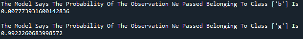
print("""The Model Says The Probability Of The Observation We Passed Belonging To Class ['b'] Is %s"""%(algorithm.predict_proba(observation)[0][0]))
print()
print("""The Model Says The Probability Of The Observation We Passed Belonging To Class ['g'] Is %s"""%(algorithm.predict_proba(observation)[0][1]))

The expected result would be the following:

Conclution.

This concludes my article. Now we understand the logic behind this supervised machine learning algorithm and we know how to implement it in a binary classification problem.

Thanks for your time.

Related