Skull removal: Image segmentation in 3D MRI images

This article was published as part of the Data Science Blogathon

Removing the skull is one of the preliminary steps on the way to detecting abnormalities in the brain.. It is the process of isolating brain tissue from non-brain tissue from an MRI image of a brain. This segmentation of the brain from the skull is a tedious task even for expert radiologists and the accuracy of the results varies greatly from person to person.. Here we are trying to automate the process by creating an end-to-end pipeline where we only need to input the raw MRI image and the pipeline should generate a segmented image of the brain after doing the necessary pre-processing..

Then, What is an MRI image?

To obtain an MRI image of a patient, are inserted into a tunnel with a magnetic field inside. This causes all the protons in the body to “line up”, so its quantum spin is the same. Then, an oscillating magnetic field pulse is used to disrupt this alignment. When the protons return to equilibrium, send out an electromagnetic wave. Depending on the fat content, the chemical composition and, what is more important, the type of stimulation (namely, the sequences) used to disrupt protons, different images will be obtained. Four common sequences that are obtained are T1, T1 with contrast (T1C), T2, Y INSTINCT.

Common challenges when working with brain imaging

• Challenges of real world data

  Building a model and achieving good accuracy on a jupyter laptop is good. But most of the time, a very good performing model performs very poorly on real world data. This happens due to data drift when the model sees completely different data than it is trained to.. In our case, it can happen due to differences in some parameters or magnetic resonance imaging methods. Here's a Blog describing some real-world AI failures.

Problem formulation

The task we have here is to give a 3D MRI image that we have to identify the brain and segment the brain tissue from the full image of a skull.. For this task, we will have a basic truth tag and, Thus, will be a supervised image segmentation task. We will use loss of dice as our loss function.

Data

Let's take a look at the dataset we will use for this task. The dataset can be downloaded from here.

The repository contains data from 125 participants, of 21 a 45 years, with a variety of clinical and subclinical psychiatric symptoms. For each participant, the repository contains:

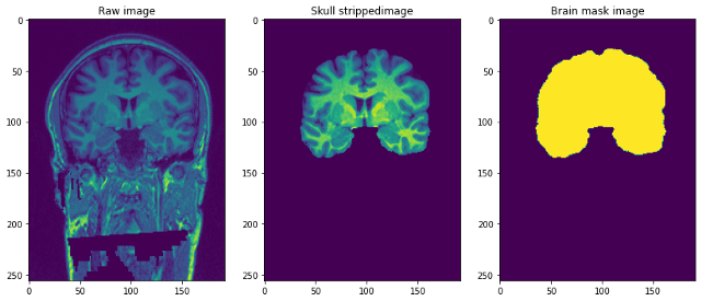
• Structural T1-weighted magnetic resonance imaging (faceless): this is raw T1 weighted MRI image with single channel.
• Brain mask: is the image mask of the brain or can it be called the fundamental truth. Obtained using the Beast method (brain extraction based on non-local segmentation) and applying manual edits by domain experts to remove non-brain tissue.
• Stripped skull image: this can be thought of as part of the brain stripped of the previous T1-weighted image. This is similar to superimposing masks on real images.

The resolution of the images is 1 mm3 and each file is in NiFTI format (.nii.gz). A single data point looks like this …

Preprocessing our Raw images

img=nib.load('/content/NFBS_Dataset/A00028185/sub-A00028185_ses-NFB3_T1w.nii.gz')
print('Shape of image=",img.shape)

Imagine 3-D images above as if we had 192 2-D sized images 256 * 256 stacked on top of each other.

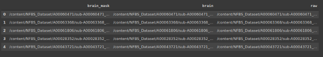
Let's create a data frame that contains the location of the images and the corresponding masks and the images without skulls.

#storing the address of 3 types of files
import os
brain_mask=[]
brain=[]
raw=[]
for subdir, dirs, files in os.walk("/content/NFBS_Dataset'):
    for file in files:
        #print os.path.join(subdir, file)y
        filepath = subdir + os.sep + file

        if filepath.endswith(".gz"):
          if '_brainmask.' in filepath:
            brain_mask.append(filepath)
          elif '_brain.' in filepath:
            brain.append(filepath)
          else:
            raw.append(filepath)

The bias field signal is a very soft, low-frequency signal that corrupts MRI images., especially those produced by old MRIs (Magnetic resonance imaging) machines. Image processing algorithms such as segmentation, texture analysis or classification using image pixel gray level values ​​will not produce satisfactory results. A preprocessing step is required to correct the polarizing field signal before sending corrupted MRI images to such algorithms or the algorithms must be modified.

• Crop and resize

  Due to computational limitations of fitting the full image to the model here, we decided to reduce the size of the MRI image from (256 * 256 * 192) a (96 * 128 * 160). The size of the target is chosen in such a way that most of the skull is captured and, after cropping and resizing it, has a centering effect on images.

• Intensity normalization

  Normalization changes and scales an image so that the pixels in the image have zero mean and unit variance. This helps the model converge faster by eliminating scale variation. Below is the code for it.

  class preprocessing():
    def __init__(self,df):
      self.data=df
      self.raw_index=[]
      self.mask_index=[]
    def bias_correction(self):
      !mkdir bias_correction
      n4 = N4BiasFieldCorrection()
      n4.inputs.dimension = 3
      n4.inputs.shrink_factor = 3
      n4.inputs.n_iterations = [20, 10, 10, 5]
      index_corr=[]
      for i in tqdm(range(len(self.data))):
        n4.inputs.input_image = self.data.raw.iloc[i]
        n4.inputs.output_image="bias_correction/"+str(i)+'.nii.gz'
        index_corr.append('bias_correction/'+str(i)+'.nii.gz')
        res = n4.run()
      index_corr=['bias_correction/'+str(i)+'.nii.gz' for i in range(125)]
      data['bias_corr']=index_corr
      print('Bias corrected images stored at : bias_correction/')
    def resize_crop(self):
      #Reducing the size of image due to memory constraints
      !mkdir resized
      target_shape = np.array((96,128,160))                   #reducing size of image from 256*256*192 to 96*128*160
      new_resolution = [2,]*3
      new_affine = np.zeros((4,4))
      new_affine[:3,:3] = np.diag(new_resolution)
      # putting point 0,0,0 in the middle of the new volume - this could be refined in the future
      new_affine[:3,3] = target_shape*new_resolution/2.*-1
      new_affine[3,3] = 1.
      raw_index=[]
      mask_index=[]
      #resizing both image and mask and storing in folder
      for i in range(len(data)):
        downsampled_and_cropped_nii = resample_img(self.data.bias_corr.iloc[i], target_affine=new_affine, target_shape=target_shape, interpolation='nearest')
        downsampled_and_cropped_nii.to_filename('resized/raw'+str(i)+'.nii.gz')
        self.raw_index.append('resized/raw'+str(i)+'.nii.gz')
        downsampled_and_cropped_nii = resample_img(self.data.brain_mask.iloc[i], target_affine=new_affine, target_shape=target_shape, interpolation='nearest')
        downsampled_and_cropped_nii.to_filename('resized/mask'+str(i)+'.nii.gz')
        self.mask_index.append('resized/mask'+str(i)+'.nii.gz')
      return self.raw_index,self.mask_index
    def intensity_normalization(self):
      for i in self.raw_index:
        image = sitk.ReadImage(i)
        resacleFilter = sitk.RescaleIntensityImageFilter()
        resacleFilter.SetOutputMaximum(255)
        resacleFilter.SetOutputMinimum(0)
        image = resacleFilter.Execute(image)
        sitk.WriteImage(image,i)
      print('Normalization done. Images stored at: resized/')

Let's take a look at the architecture of the model.

  def data_gen(self,img_list, mask_list, batch_size):
    '''Custom data generator to feed image to model'''
    c = 0
    n = [i for i in range(len(img_list))]  #List of training images
    random.shuffle(n)
    
    while (True):
      img = np.zeros((batch_size, 96, 128, 160,1)).astype('float')   #adding extra dimensions as conv3d takes file of size 5
      mask = np.zeros((batch_size, 96, 128, 160,1)).astype('float')

      for i in range(c, c+batch_size): 
        train_img = nib.load(img_list[n[i]]).get_data()
        
        train_img=np.expand_dims(train_img,-1)
        train_mask = nib.load(mask_list[n[i]]).get_data()

        train_mask=np.expand_dims(train_mask,-1)

        img[i-c]=train_img
        mask[i-c] = train_mask
      c+=batch_size
      if(c+batch_size>= len(img_list)):
        c=0
        random.shuffle(n)

      yield img,mask

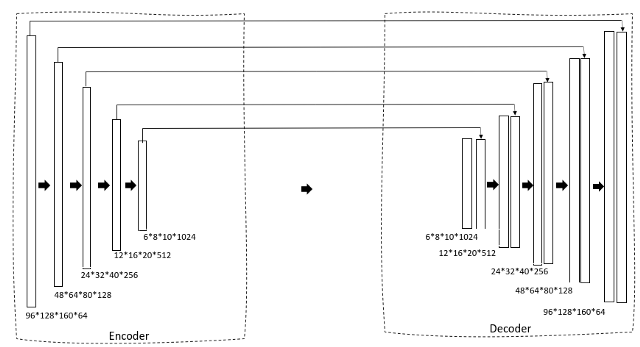
We are using a U-Net 3D as our architecture. If you are already familiar with the U-Net 2D, this will be very simple. First, we have a shrink path through an encoder that gradually reduces the image size and increases the number of filters to generate bottleneck characteristics. This is then fed to a decoder block which gradually expands the size so that it can finally generate a mask as the intended output.

  def convolutional_block(input, filters=3, kernel_size=3, batchnorm = True):
    '''conv layer followed by batchnormalization'''
    x = Conv3D(filters = filters, kernel_size = (kernel_size, kernel_size,kernel_size),
               kernel_initializer="he_normal", padding = 'same')(input)
    if batchnorm:
        x = BatchNormalization()(x)
    x = Activation('relu')(x)
    x = Conv3D(filters = filters, kernel_size = (kernel_size, kernel_size,kernel_size),
               kernel_initializer="he_normal", padding = 'same')(input)
    if batchnorm:
        x = BatchNormalization()(x)
    x = Activation('relu')(x) 
    return x

def resunet_opt(input_img, filters = 64, dropout = 0.2, batchnorm = True):
    """Residual 3D Unet"""
    conv1 = convolutional_block(input_img, filters * 1, kernel_size = 3, batchnorm = batchnorm)
    pool1 = MaxPooling3D((2, 2, 2))(conv1)
    drop1 = Dropout(dropout)(pool1)

    conv2 = convolutional_block(drop1, filters * 2, kernel_size = 3, batchnorm = batchnorm)
    pool2 = MaxPooling3D((2, 2, 2))(conv2)
    drop2 = Dropout(dropout)(pool2)

    conv3 = convolutional_block(drop2, filters * 4, kernel_size = 3, batchnorm = batchnorm)
    pool3 = MaxPooling3D((2, 2, 2))(conv3)
    drop3 = Dropout(dropout)(pool3)

    conv4 = convolutional_block(drop3, filters * 8, kernel_size = 3, batchnorm = batchnorm)
    pool4 = MaxPooling3D((2, 2, 2))(conv4)
    drop4 = Dropout(dropout)(pool4)

    conv5 = convolutional_block(drop4, filters = filters * 16, kernel_size = 3, batchnorm = batchnorm)
    conv5 = convolutional_block(conv5, filters = filters * 16, kernel_size = 3, batchnorm = batchnorm)
    
    ups6 = Conv3DTranspose(filters * 8, (3, 3, 3), strides = (2, 2, 2), padding = 'same',activation = 'reread',kernel_initializer="he_normal")(conv5)
    ups6 = concatenate([ups6, conv4])
    ups6 = Dropout(dropout)(ups6)
    conv6 = convolutional_block(ups6, filters * 8, kernel_size = 3, batchnorm = batchnorm)

    ups7 = Conv3DTranspose(filters * 4, (3, 3, 3), strides = (2, 2, 2), padding = 'same',activation = 'reread',kernel_initializer="he_normal")(conv6)
    ups7 = concatenate([ups7, conv3])
    ups7 = Dropout(dropout)(ups7)
    conv7 = convolutional_block(ups7, filters * 4, kernel_size = 3, batchnorm = batchnorm)

    ups8 = Conv3DTranspose(filters * 2, (3, 3, 3), strides = (2, 2, 2), padding = 'same',activation = 'reread',kernel_initializer="he_normal")(conv7)
    ups8 = concatenate([ups8, conv2])
    ups8 = Dropout(dropout)(ups8)
    conv8 = convolutional_block(ups8, filters * 2, kernel_size = 3, batchnorm = batchnorm)
    
    ups9 = Conv3DTranspose(filters * 1, (3, 3, 3), strides = (2, 2, 2), padding = 'same',activation = 'reread',kernel_initializer="he_normal")(conv8)
    ups9 = concatenate([ups9, conv1])
    ups9 = Dropout(dropout)(ups9)
    conv9 = convolutional_block(ups9, filters * 1, kernel_size = 3, batchnorm = batchnorm)
    
    outputs = Conv3D(1, (1, 1, 2), activation='sigmoid',padding='same')(conv9)
    model = model(inputs=[input_img], outputs=[outputs])
    return model

We then train the model using Adam's optimizer and loss of dice as our loss function …

  def training(self,epochs):
    im_height=96
    im_width=128
    img_depth=160
    epochs=60
    train_gen = data_gen(self.X_train,self.y_train, batch_size = 4)
    val_gen = data_gen(self.X_test,self.y_test, batch_size = 4)
    channels=1
    input_img = Input((im_height, im_width,img_depth,channels), name="img")
    self.model = resunet_opt(input_img, filters=16, dropout=0.05, batchnorm=True)
    self.model.summary()
    self.model.compile(optimizer=Adam(lr=1e-1),loss=focal_loss,metrics=[iou_score,'accuracy'])
    #fitting the model
    callbacks=callbacks = [
        ModelCheckpoint('best_model.h5', verbose=1, save_best_only=True, save_weights_only=False)]
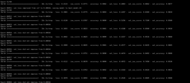
    result=self.model.fit(train_gen,steps_per_epoch=16,epochs=epochs,validation_data=val_gen,validation_steps=16,initial_epoch=0,callbacks=callbacks)

After training for 60 epochs, we got a validation iou_score from 0.86.

Let's take a look at how our model worked. Our model will simply predict the mask. To get the image without skull, we need to overlay it on the Raw image to get the image without skull …

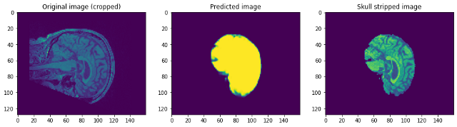
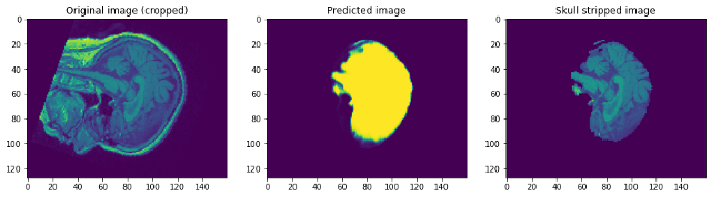
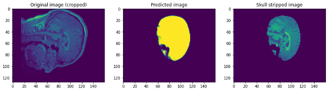
Looking at the predictions we can say that although it is able to identify the brain and segment it, not close to perfection. In this point, we can sit down with a domain expert to identify what additional preprocessing steps can be taken to improve accuracy. But as for this post, I will conclude it here. Please, follow link1 Y / O link2 If you want to know more …

Conclution:

I'm glad you made it to the end. Hope this helps you get started with image segmentation into 3D images. You can find the Google Colab link that contains the code. here. Feel free to add suggestions or queries in the comment section. Have a nice day!

Media shown in this skull removal article is not the property of DataPeaker and is used at the author's discretion.

Related