Introduction
Deep learning is rapidly gaining traction as more and more research articles emerge from around the world.. Undoubtedly, these documents contain a lot of information, but they can often be difficult to analyze. And to understand them, you may have to review that document multiple times (And maybe even other dependent documents!).
This is truly a daunting task for non-academics like us..

Personally, I find the task to review a research article, interpret the crux behind it and implement the code as an important skill that every deep learning enthusiast and practitioner should possess. The practical implementation of research ideas brings out the author's thought process and also helps transform those ideas into real-world industry applications..
Then, in this article (and the following series of articles) my reason for writing is twofold:
- Let readers keep up with cutting edge research by breaking down deep learning articles into understandable concepts.
- Learn to code research ideas for myself and encourage people to do so simultaneously.
This article assumes you have a good understanding of the basics of deep learning.. In case you don't need it, or just need a refresher, check the items below first then come back here soon:
Table of Contents
- Document Summary “Delve into convolutions”
- Objective of the work
- Proposed architectural details
- Training methodology
- GoogLeNet implementation in Keras
Document Summary “Delve into convolutions”
This article focuses on paper “Dig Deeper with Convolutions” where the distinctive idea of the homenet came from. The home network was once considered an architecture (the model) next-generation deep learning tool to solve image recognition and detection problems.
Featured groundbreaking performance in the ImageNet Visual Recognition Challenge (in 2014), which is a renowned platform for benchmarking image recognition and detection algorithms. along with this, a lot of research was started on creating new deep learning architectures with innovative and impactful ideas.
We will review the main ideas and suggestions proposed in the document mentioned above and try to understand the techniques it contains. In the words of the author:
“In this article, we will focus on an efficient deep neural network architecture for computer vision, whose code name is Inception, which derives its name from (…) the famous internet meme” we need to go deeper “.

That sounds intriguing, ¿no? Good, Keep reading then!
Objective of the work
There is a simple but powerful way to create better deep learning models. You can just make a bigger model, either in terms of depth, namely, number of layers, or the number of neurons in each layer. But how can you imagine, this can often create complications:
- The bigger the model, more prone to over-adjusting. This is particularly noticeable when the training data is small..
- Increasing the number of parameters means that you need to increase your existing computational resources
A solution for this, as the document suggests, is to move to loosely connected network architectures that will replace fully connected network architectures, especially within convolutional layers. This idea can be conceptualized in the following images:
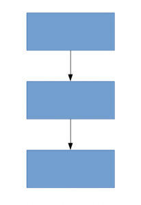
Densely connected architecture
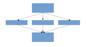
Sparsely connected architecture
This article proposes a new idea of creating deep architectures. This approach allows you to maintain “computational budget”, while increasing the depth and width of the net. It sounds too good to be true! This is what the conceptualized idea looks like:
Let's look at the proposed architecture in a little more detail.
Proposed architectural details
The document proposes a new type of architecture: GoogLeNet o Inception v1. It is basically a convolutional neural network (CNN) what's wrong with it 27 layers deep.. Below is the summary of the model:
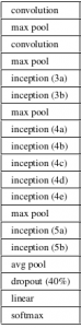
Notice in the image above that there is a layer called the start layer. This is actually the main idea behind the focus of the document. The initial layer is the central concept of a loosely connected architecture.
Idea of a starter module
Let me explain in a little more detail what a startup layer is all about. Taking an excerpt from the article:
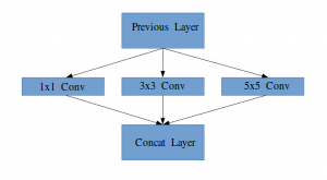
“(Start layer) it's a combination of all those layers (namely, convolutional cover 1 × 1, convolutional cover 3 × 3, convolutional cover 5 × 5) with their output filter banks concatenated into a single output vector that forms the input of the following scenario.”
Along with the layers mentioned above, there are two main plugins in the original start layer:
- convolutional cover 1 × 1 before applying another coat, which is mainly used for dimensionality reduction
- A parallel maximum grouping layer, which provides another option to the start layer

Start layer
To understand the importance of the structure of the initial layer, the author draws on the Hebbian principle of human learning. This says that “neurons firing together, they connect together”. The author suggests that When creating a post layer in a deep learning model, attention should be paid to the learnings from the previous layer.
Suppose, for instance, that one layer of our deep learning model has learned to focus on individual parts of a face. The next layer of the network would probably focus on the general face of the image to identify the different objects present there. Now, to do this, the layer must have the appropriate filter sizes to detect different objects.
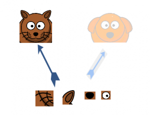
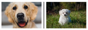
This is where the initial layer comes to the fore. Allows inner layers to pick and choose which filter size will be relevant to know the required information. Then, even if the size of the face in the picture is different (as seen in the pictures below), the cape works accordingly to recognize the face. For the first image, you would probably need a higher filter size, while I would take a lower one for the second image.
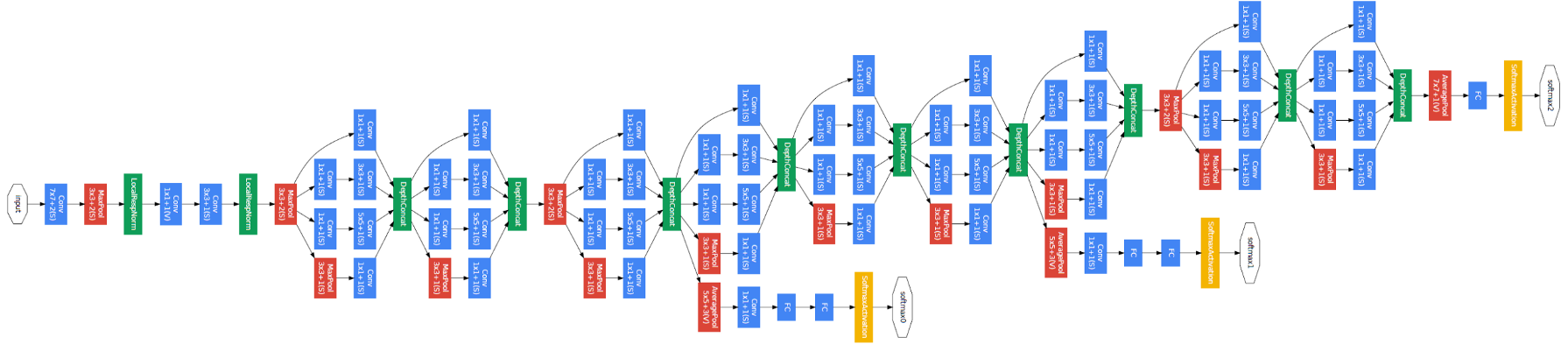
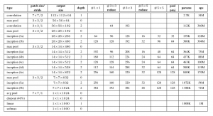
General architecture, with all specifications, it looks like this:
Training methodology
Note that this architecture arose in large part because the authors participated in an image detection and recognition challenge.. Therefore, there are plenty “bells and whistles” that they have explained in the document. These include:
- The hardware they used to train the models.
- The data augmentation technique to create the training dataset.
- The hyperparameters of the neural network, such as the optimization technique and the learning rate program.
- Auxiliary training required to train the model.
- Assembly techniques they used to build the final presentation.
Between these, the auxiliary training carried out by the authors is quite interesting and novel by nature. So we'll focus on that for now.. The details of the rest of the techniques can be taken from the article itself, or in the implementation that we will see below.
To prevent the middle part of the network from "disappearing", the authors introduced two auxiliary classifiers (the purple squares in the image). Basically, applied softmax to the outputs of two of the starter modules and calculated an auxiliary loss on the same labels. The total loss function is a weighted sum of the auxiliary loss and the actual loss. The weight value used on the paper was 0,3 for each auxiliary loss.
GoogLeNet implementation in Keras
Now that you have understood the GoogLeNet architecture and the intuition behind it, It's time to fire up Python and implement our learnings using Keras!! We will use the CIFAR-10 dataset for this purpose.
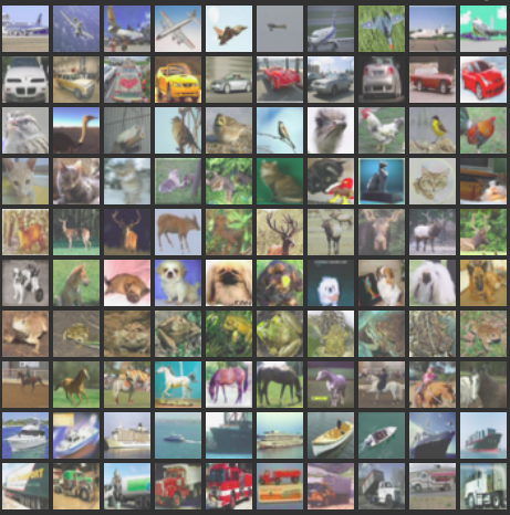
CIFAR-10 is a popular image classification data set. It consists of 60.000 images of 10 lessons (each class is represented as a row in the image above). The data set is divided into 50.000 training images and 10.000 test images.
Keep in mind that you must have the necessary libraries installed to implement the code that we will see in this section. This includes Keras and TensorFlow (as backend for Keras). You can check the official installation guide in case you don't have Keras already installed on your machine.
Now that we have taken care of the prerequisites, we can finally start coding the theory we covered in the previous sections. The first thing we must do is import all the necessary libraries and modules that we will use throughout the code.
import hard
from hard.layers.core import Layer
import keras.backend as K
import tensorflow as tf
from hard.datasets import cifar10
from hard.models import Model
from hard.layers import Conv2D, MaxPool2D,
    Dropout, Dense, Input, concatenate,
    GlobalAveragePooling2D, AveragePooling2D,
    Flatten

import cv2
import numpy as e.g
from hard.datasets import cifar10
from hard import backend as K
from hard.utils import np_utils

import math
from hard.optimizers import SGD
from loud.callbacks import LearningRateScheduler
Then we will load the dataset and do some preprocessing steps. This is a critical task before the deep learning model is trained.
num_classes = 10

def load_cifar10_data(img_rows, img_cols):

    # Load cifar10 training and validation sets
    (X_train, Y_train), (X_valid, Y_valid) = cifar10.load_data()

    # Resize training images
    X_train = e.g.array([cv2.resize(img, (img_rows,img_cols)) for img in X_train[:,:,:,:]])
    X_valid = e.g.array([cv2.resize(img, (img_rows,img_cols)) for img in X_valid[:,:,:,:]])

    # Transform targets to keras compatible format
    Y_train = np_utils.to_categorical(Y_train, num_classes)
    Y_valid = np_utils.to_categorical(Y_valid, num_classes)

    X_train = X_train.astype('float32')
    X_valid = X_valid.astype('float32')

    # preprocess data
    X_train = X_train / 255.0
    X_valid = X_valid / 255.0

    return X_train, Y_train, X_valid, Y_valid
X_train, y_train, X_test, y_test = load_cifar10_data(224, 224)
Now, we will define our deep learning architecture. We will quickly define a function to do this, that, when you are given the necessary information, returns us the entire start layer.
def inception_module(x,
                     filters_1x1,
                     filters_3x3_reduce,
                     filters_3x3,
                     filters_5x5_reduce,
                     filters_5x5,
                     filters_pool_proj,
                     name=None):

    conv_1x1 = Conv2D(filters_1x1, (1, 1), padding='same', activation='relu', kernel_initializer=kernel_init, bias_initializer=bias_init)(x)

    conv_3x3 = Conv2D(filters_3x3_reduce, (1, 1), padding='same', activation='relu', kernel_initializer=kernel_init, bias_initializer=bias_init)(x)
    conv_3x3 = Conv2D(filters_3x3, (3, 3), padding='same', activation='relu', kernel_initializer=kernel_init, bias_initializer=bias_init)(conv_3x3)

    conv_5x5 = Conv2D(filters_5x5_reduce, (1, 1), padding='same', activation='relu', kernel_initializer=kernel_init, bias_initializer=bias_init)(x)
    conv_5x5 = Conv2D(filters_5x5, (5, 5), padding='same', activation='relu', kernel_initializer=kernel_init, bias_initializer=bias_init)(conv_5x5)

    pool_proj = MaxPool2D((3, 3), strides=(1, 1), padding='same')(x)
    pool_proj = Conv2D(filters_pool_proj, (1, 1), padding='same', activation='relu', kernel_initializer=kernel_init, bias_initializer=bias_init)(pool_proj)

    output = concatenate([conv_1x1, conv_3x3, conv_5x5, pool_proj], axis=3, name=name)

    return output
Then we will create the GoogLeNet architecture, as mentioned in the document.
kernel_init = hard.initializers.glorot_uniform()
bias_init = hard.initializers.Constant(value=0.2)
input_layer = Input(shape=(224, 224, 3))

x = Conv2D(64, (7, 7), padding='same', strides=(2, 2), activation='relu', name='conv_1_7x7/2', kernel_initializer=kernel_init, bias_initializer=bias_init)(input_layer)
x = MaxPool2D((3, 3), padding='same', strides=(2, 2), name='max_pool_1_3x3/2')(x)
x = Conv2D(64, (1, 1), padding='same', strides=(1, 1), activation='relu', name='conv_2a_3x3/1')(x)
x = Conv2D(192, (3, 3), padding='same', strides=(1, 1), activation='relu', name='conv_2b_3x3/1')(x)
x = MaxPool2D((3, 3), padding='same', strides=(2, 2), name='max_pool_2_3x3/2')(x)

x = inception_module(x,
                     filters_1x1=64,
                     filters_3x3_reduce=96,
                     filters_3x3=128,
                     filters_5x5_reduce=16,
                     filters_5x5=32,
                     filters_pool_proj=32,
                     name='inception_3a')

x = inception_module(x,
                     filters_1x1=128,
                     filters_3x3_reduce=128,
                     filters_3x3=192,
                     filters_5x5_reduce=32,
                     filters_5x5=96,
                     filters_pool_proj=64,
                     name='inception_3b')

x = MaxPool2D((3, 3), padding='same', strides=(2, 2), name='max_pool_3_3x3/2')(x)

x = inception_module(x,
                     filters_1x1=192,
                     filters_3x3_reduce=96,
                     filters_3x3=208,
                     filters_5x5_reduce=16,
                     filters_5x5=48,
                     filters_pool_proj=64,
                     name='inception_4a')


x1 = AveragePooling2D((5, 5), strides=3)(x)
x1 = Conv2D(128, (1, 1), padding='same', activation='relu')(x1)
x1 = Flatten()(x1)
x1 = Dense(1024, activation='relu')(x1)
x1 = Dropout(0.7)(x1)
x1 = Dense(10, activation='softmax', name='auxilliary_output_1')(x1)

x = inception_module(x,
                     filters_1x1=160,
                     filters_3x3_reduce=112,
                     filters_3x3=224,
                     filters_5x5_reduce=24,
                     filters_5x5=64,
                     filters_pool_proj=64,
                     name='inception_4b')

x = inception_module(x,
                     filters_1x1=128,
                     filters_3x3_reduce=128,
                     filters_3x3=256,
                     filters_5x5_reduce=24,
                     filters_5x5=64,
                     filters_pool_proj=64,
                     name='inception_4c')

x = inception_module(x,
                     filters_1x1=112,
                     filters_3x3_reduce=144,
                     filters_3x3=288,
                     filters_5x5_reduce=32,
                     filters_5x5=64,
                     filters_pool_proj=64,
                     name='inception_4d')


x2 = AveragePooling2D((5, 5), strides=3)(x)
x2 = Conv2D(128, (1, 1), padding='same', activation='relu')(x2)
x2 = Flatten()(x2)
x2 = Dense(1024, activation='relu')(x2)
x2 = Dropout(0.7)(x2)
x2 = Dense(10, activation='softmax', name='auxilliary_output_2')(x2)

x = inception_module(x,
                     filters_1x1=256,
                     filters_3x3_reduce=160,
                     filters_3x3=320,
                     filters_5x5_reduce=32,
                     filters_5x5=128,
                     filters_pool_proj=128,
                     name='inception_4e')

x = MaxPool2D((3, 3), padding='same', strides=(2, 2), name='max_pool_4_3x3/2')(x)

x = inception_module(x,
                     filters_1x1=256,
                     filters_3x3_reduce=160,
                     filters_3x3=320,
                     filters_5x5_reduce=32,
                     filters_5x5=128,
                     filters_pool_proj=128,
                     name='inception_5a')

x = inception_module(x,
                     filters_1x1=384,
                     filters_3x3_reduce=192,
                     filters_3x3=384,
                     filters_5x5_reduce=48,
                     filters_5x5=128,
                     filters_pool_proj=128,
                     name='inception_5b')

x = GlobalAveragePooling2D(name='avg_pool_5_3x3/1')(x)

x = Dropout(0.4)(x)

x = Dense(10, activation='softmax', name='output')(x)
model = Model(input_layer, [x, x1, x2], name='inception_v1')
Let's summarize our model to check if our work so far has gone well.
The model looks good, as you can measure from the above output. We can add some finishing touches before training our model. We will define the following:
- Loss function for each output layer
- Weight assigned to that output layer
- Optimization function, which is modified to include a decrease in weight after each 8 epochs.
- Evaluation metric
epochs = 25
initial_lrate = 0.01

def decay(epoch, steps=100):
    initial_lrate = 0.01
    drop = 0.96
    epochs_drop = 8
    lrate = initial_lrate * math.pow(drop, math.floor((1+epoch)/epochs_drop))
    return lrate

sgd = SGD(lr=initial_lrate, momentum=0.9, nesterov=False)

lr_sc = LearningRateScheduler(decay, verbose=1)

model.compile(loss=['categorical_crossentropy', 'categorical_crossentropy', 'categorical_crossentropy'], loss_weights=[1, 0.3, 0.3], optimizer=sgd, metrics=['accuracy'])
Our model is now ready! Give it a try to see how it works.
history = model.fit(X_train, [y_train, y_train, y_train], validation_data=(X_test, [y_test, y_test, y_test]), epochs=epochs, batch_size=256, callbacks=[lr_sc])
Below is the result I got when training the model:
Our model gave impressive precision of the 80% + in the validation set, which shows that this model architecture is really worth checking out.
Final notes
This was a really nice article to write and I hope you found it equally useful. Inception v1 was the focal point of this article, in which I explained the nitty-gritty of this framework and demonstrated how to implement it from scratch in Keras.
In the next articles, I will focus on advances in Inception architectures. These advances were detailed in later articles., namely, Inception v2, Inception v3, etc. And if, they are as intriguing as the name suggests, So stay tuned!
If you have any suggestions / comment related to the article, post it in the comment section below.


