This article was published as part of the Data Science Blogathon
Introduction
Feature selection is the process of selecting features that are relevant to a machine learning model. It means that it selects only those attributes that have a significant effect on the model output.
Consider the case when you go to the department store to buy groceries. A product has a lot of information, namely, product, category, due date, MRP, ingredients and manufacturing details. All this information is the characteristics of the product. Normally, check the brand, the MRP and expiration date before purchasing a product. But nevertheless, the ingredients and manufacturing section is none of your concern. Therefore, the brand, el mrp, the expiration date are relevant characteristics and the ingredient, manufacturing details are irrelevant. This is how feature selection is done.
In the real world, a dataset can have thousands of features and there may be chances that some features are redundant, some may be correlated and some may be irrelevant to the model. In this stage, if you use all functions, it will take a long time to train the model and the accuracy of the model will be reduced. Therefore, feature selection becomes important in model building. There are many other ways to select features, as elimination of recursive features, genetic algorithms, decision trees. But nevertheless, I will tell you the most basic and manual method of filtering using statistical tests.
Now that you have a basic understanding of feature selection, we will see how to implement various statistical tests on the data to select important characteristics.
Target
The main objective of this blog is to understand statistical tests and their implementation in real data in Python, which will help in the selection of features.
Terminologies
Before getting into the types of statistical tests and their implementation, you need to understand the meanings of some terminologies.
Hypothesis testing
Hypothesis testing in statistics is a method of testing the results of experiments or surveys to see if it has meaningful results.. Useful when you want to infer about a population based on a sample or correlation between two or more samples.
Null hypothesisThe null hypothesis is a fundamental concept in statistics that establishes an initial statement about a population parameter. Its purpose is to be tested and, if refuted, allows us to accept the alternative hypothesis. This approach is essential in scientific research, as it provides a framework for evaluating empirical evidence and making data-driven decisions. Its formulation and analysis are crucial in statistical studies....
This hypothesis establishes that there is no significant difference between sample and population or between different populations.. It is denoted by H0.
Not. We assume that the mean of 2 samples is the same.
Alternative hypothesis
The statement contrary to the null hypothesis is included in the alternative hypothesis. It is denoted by H1.
Not. We assume that the mean of the 2 samples is uneven.
critical value
It is a point on the scale of the test statistic beyond which the null hypothesis is rejected.. The higher the critical value, the lower the probability that 2 samples belong to the same distribution. The critical value for any test can
p value
p-value means 'probability value'; indicates the probability that an outcome occurred by chance. Basically, the p-value is used in hypothesis testing to help you support or reject the null hypothesis. The smaller the p-value, the stronger the evidence to reject the null hypothesis.
Degree of freedom
The degree of freedom is the number of independent variables. This concept is used to calculate the t statistic and the chi-square statistic.
You may refer to statisticswho.com for more information on these terminologies.
Statistical tests
Una prueba estadística es una forma de determinar si la variableIn statistics and mathematics, a "variable" is a symbol that represents a value that can change or vary. There are different types of variables, and qualitative, that describe non-numerical characteristics, and quantitative, representing numerical quantities. Variables are fundamental in experiments and studies, since they allow the analysis of relationships and patterns between different elements, facilitating the understanding of complex phenomena.... aleatoria sigue la hipótesis nula o la hipótesis alternativa. Basically, says if the sample and the population or two or more samples have significant differences. You can use various descriptive statistics as average, medianThe median is a statistical measure that represents the central value of a set of ordered data. To calculate it, the data is organized from lowest to highest and the number in the middle is identified. If there are an even number of observations, the two core values are averaged. This indicator is especially useful in asymmetric distributions, since it is not affected by extreme values...., way, range or standard deviation for this purpose. But nevertheless, we generally use the mean. The statistical test gives you a number which is then compared to the p-value. If its value is greater than the p-value, accept the null hypothesis, on the contrary, She rejects.
The procedure to implement each statistical test will be as follows:
- We calculate the statistical value using the mathematical formula
- Then we calculate the critical value using statistical tables.
- With the help of critical value, we calculate the p-value
- If the p-value> 0.05 we accept the null hypothesis, otherwise we reject it
Now that you understand feature selection and statistical testing, we can move towards the implementation of various statistical tests along with their meaning. Before that, i will show you the dataset and this dataset will be used for all testing.
Data set
The dataset I will be using is a loan prediction dataset that was taken from the Vidhya analysis contest. You can also participate in the contest and download the data set. here.
First I imported all the necessary python modules and the dataset.
import numpy as np
import pandas as pd
import seaborn as sb
from numpy import sqrt, abs, round
import scipy.stats as stats
from scipy.stats import norm
df=pd.read_csv('loan.csv')
df.head()
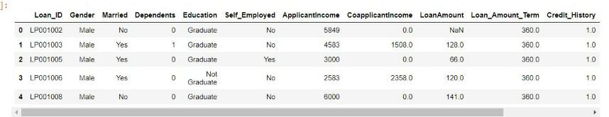
There are many characteristics in the dataset, as gender, dependents, education, applicant's income, loan amount, credit history. We will use these features and check if one feature effect affects other features using various tests, namely, Z test, correlation test, ANOVA test and Chi-square test.
Z test
A Z test is used to compare the mean of two given samples and infer whether they belong to the same distribution or not.. We do not implement the Z test when the sample size is less than 30.
A Z-test can be a one-sample Z-test or a two-sample Z-test.
The unique sample test t determines whether the sample mean is statistically different from a known or hypothesized population mean. The two-sample Z test compares 2 independent variables.
We will implement a two-sample Z-test.
The Z statistic is denoted by

Implementation
Please note that we will implement 2 sample z tests where one variable will be categorical with two categories and the other variable will be continuous to apply the z test.
Here we will use the Gender categorical variable and Applicant Income Continuous variable. The genre has 2 groups: male and female. Therefore the hypothesis will be:
Null hypothesis: There is no significant difference between the mean income of men and women.
Alternative hypothesis: there is a significant difference between the mean income of men and women.
Code
M_mean=df.loc[df['Gender']=='Male','ApplicantIncome'].mean()
F_mean=df.loc[df['Gender']=='Female','ApplicantIncome'].mean()
M_std=df.loc[df['Gender']=='Male','ApplicantIncome'].std()
F_std=df.loc[df['Gender']=='Female','ApplicantIncome'].std()
no_of_M=df.loc[df['Gender']=='Male','ApplicantIncome'].count()
no_of_F=df.loc[df['Gender']=='Female','ApplicantIncome'].count()
The above code calculates the mean income of male applicants, the mean income of female applicants, its standard deviation and the number of samples of men and women.
twoSampZ La función calculará la estadística z y el valor p sin pasar por los parametersThe "parameters" are variables or criteria that are used to define, measure or evaluate a phenomenon or system. In various fields such as statistics, Computer Science and Scientific Research, Parameters are critical to establishing norms and standards that guide data analysis and interpretation. Their proper selection and handling are crucial to obtain accurate and relevant results in any study or project.... de entrada calculados anteriormente.
def twoSampZ(X1, X2, mudiff, sd1, sd2, n1, n2):
    pooledSE = sqrt(sd1**2/n1 + sd2**2/n2)
    z = ((X1 - X2) - mudiff)/pooledSE
    pval = 2*(1 - norm.cdf(abs(With)))
    return round(With,3), pval
z,p= twoSampZ(M_mean,F_mean,0,M_std,F_std,no_of_M,no_of_F)
print('Z'= z,'p'= p)
Z = 1.828
p = 0.06759726635832197
if p<0.05:
    print("we reject null hypothesis")
else:
    print("we accept null hypothesis")
we accept the null hypothesis
Since the p-value is greater than 0.5 we accept the null hypothesis. Therefore, we conclude that there is no significant difference between the income of men and women.
Test T
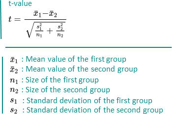
A t-test is also used to compare the mean of two given samples., like Z test. But nevertheless, is implemented when the sample size is less than 30. A normal distribution of the sample is assumed. It can also be one or two samples. The degree of freedom is calculated by n-1 where n is the number of samples.
It is denoted by
Implementation
It will be implemented in the same way as the Z test. The only condition is that the sample size must be less than 30. I have shown you the implementation of the Z test. Now, you can try the T-Test.
Correlation test
A correlation test is a metric to evaluate the extent to which variables are associated with each other.
Note that the variables must be continuous to apply the correlation test.
There are several methods for correlation testing, namely, covarianza, Pearson's correlation coefficient, Spearman's rank correlation coefficient, etc.
We will use the correlation coefficient of people since it is independent of the values of the variables.
Pearson's correlation coefficient
It is used to measure the linear correlation between 2 variables. It is denoted by
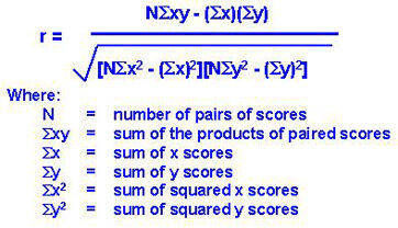
google image
Its values are between -1 Y 1.
If the value of r is 0, means that there is no relationship between the variables X and Y.
If the value of r is between 0 Y 1, means that there is a positive relationship between X and Y, and his strength increases from 0 a 1. Positive relationship means that if the value of X increases, the value of Y also increases.
If the value of r is between -1 Y 0, means there is a negative relationship between X and Y, and its strength decreases from -1 a 0. Negative relationship means that if the value of X increases, the value of Y decreases.
Implementation
Here we will use two variables or continuous characteristics: Loan amount Y Applicant income. We will conclude if there is a linear relationship between the loan amount and the applicant's income with the value of the Pearson correlation coefficient and we will also plot the graph between them.
Code
There are some missing values in the LoanAmount column, first, we fill it with the mean value. Then he calculated the value of the correlation coefficient.
df[‘LoanAmount’]= df[‘LoanAmount’].fillna (df[‘LoanAmount’].to mean())
pcc = e.g. corrcoef (df.ApplicantIncome, df.LoanAmount)
to print (pcc)
[[1.         0.56562046]
 [0.56562046 1.        ]]
The values of the diagonals indicate the correlation of characteristics with themselves. 0.56 represent that there is some correlation between the two characteristics.
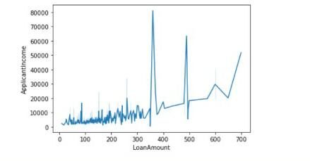
We can also draw the graph as follows:
sns.lineplot(data=df,x='LoanAmount',y = 'ApplicantIncome')
ANOVA test
ANOVA means Analysis of variance. As the name suggests, uses variance as a parameter to compare multiple independent groups. ANOVA can be unidirectional ANOVA or bidirectional ANOVA. One-way ANOVA is applied when there are three or more independent groups of one variable. We will implement the same in Python.
The F statistic can be calculated by
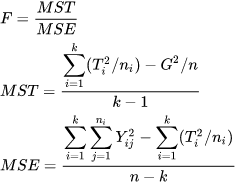
Implementation
Here we will use the Dependents categorical variable and Applicant Income Continuous variable. The dependents have 4 groups: 0,1,2,3+. Therefore the hypothesis will be:
Null hypothesis: There is no significant difference between the mean income between the different groups of dependents.
Alternative hypothesis: there is a significant difference between the mean income between the different groups of dependents.
Code
First, we handle the missing values in the Dependents function.
df['Dependents'].isnull().sum()
df['Dependents']=df['Dependents'].fillna('0')
After that, we create a data frame with the characteristics Dependents and ApplicantIncome. Later, with the help of the scipy.stats library, we calculate the F statistic and the p-value.
df_anova = df[['total_bill','day']]
grps = pd.unique(df.day.values)
d_data = {grp:df_anova['total_bill'][df_anova.day == grp] for grp in grps}
F, p = stats.f_oneway(d_data['Sun'], d_data['Sat'], d_data['Thur'],d_data['Fri'])
print('F ={},p={}'.format(F,p))
F =5.955112389949444,p=0.0005260114222572804
and P <0,05:
to print (“reject null hypothesis”)
the rest:
to print (“accept null hypothesis”)
Reject null hypothesis.
Since the p-value is less than 0.5 we reject the null hypothesis. Therefore, we conclude that there is a significant difference between the income of various groups of Dependents.
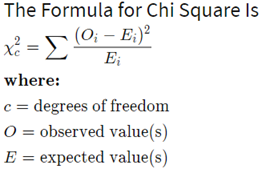
Chi-square test
This test is applied when you have two categorical variables from a population. It is used to determine if there is a significant association or relationship between the two variables.
There is 2 types of chi-square tests: chi-square goodness of fit and chi-square test for independence, we will implement the latter.
The degree of freedom in the chi-square test is calculated by (n-1) * (m-1) where n and m are numbers of rows and columns respectively.
It is denoted by:
Implementation
We will use categorical characteristics Gender Y Loan status and find out if there is an association between them using the chi-square test.
Null hypothesis: there is no significant association between gender characteristics and loan status.
Alternative hypothesis: there is a significant association between gender characteristics and loan status.
Code
First, we retrieve the column Gender and LoanStatus and form an array.
dataset_table=pd.crosstab(dataset['sex'],dataset['smoker'])
dataset_table
Loan_Status  N  Y
Gender
Female      37   75
Male        33  339
Later, we calculate the observed and expected values using the table above.
observed=dataset_table.values
val2=stats.chi2_contingency(dataset_table)
expected=val2[3]
Then we calculate the chi-square statistic and the p-value using the following code:
from scipy.stats import chi2
chi_square=sum([(o-and)**2./e for o,e in zip(observed,expected)])
chi_square_statistic=chi_square[0]+chi_square[1]
p_value=1-chi2.cdf(x=chi_square_statistic,df = ddof)
print("chi-square statistic:-",chi_square_statistic)

print('Significance level: ',alpha)

print('Degree of Freedom: ',I will come)

print('p-value:',p_value)
chi-square statistic:- 0.23697508750826923
Significance level:  0.05
Degree of Freedom:  1
p-value: 0.6263994534115932
if p_value<=alpha:

    print("Reject Null Hypothesis")

else:

    print("Accept Null Hypthesis")
Accept Null Hypthesis
Since the p-value is greater than 0.05, we accept the null hypothesis. We conclude that there is no significant association between the two characteristics.
Summary
First, we have discussed the selection of functions. Then we move on to the statistical tests and various terminologies related to it.. Finally, we have seen the application of statistical tests, namely, Z test, T test, correlation test, ANOVA and Chi-square test together with its implementation in Python.
References
Outstanding image – Google Image
Stats – statisticswho.com
About me
Hello! Soy Ashish Choudhary. I am studying B.Tech from JC Bose University of Science and Technology. Data science is my passion and I take pride in writing interesting blogs related to it. Feel free to contact me on LinkedIn.
The media shown in this article is not the property of DataPeaker and is used at the author's discretion.