This article was published as part of the Data Science Blogathon
Introduction
Sentiment analysis refers to identifying and classifying the feelings that are expressed in the source of the text. Tweets are often useful for generating a large amount of sentiment data after analysis. This data is useful for understanding people's opinion on a variety of topics..
Therefore, we need to develop a Automated Machine Learning Sentiment Analysis Model to calculate customer perception. Due to the presence of non-useful characters (collectively referred to as noise) along with useful data, difficult to implement models in them.
In this article, our goal is to analyze the sentiment of the tweets provided from the Sentiment140 data set by developing a machine learning pipeline that involves the use of three classifiers (Logistic regression, Bernoulli Naive Bayes y SVM) along with the use Term Frequency – Reverse document frequency (TF-IDF). The performance of these classifiers is then evaluated using precision Y F1 scores.

Image source: Google images
Problem Statement
In this project, we try to implement a Twitter sentiment analysis model which helps overcome the challenges of identifying sentiment from tweets. The details needed regarding the dataset are:
The data set provided is the Sentiment140 data set consisting of 1,600,000 tweets that have been extracted using the Twitter API. The various columns present in the dataset are:
- objective: the polarity of the tweet (positive or negative)
- identifiers: Unique tweet ID
- date: the date of the tweet
- flag: Refers to the query. If there is no such query, then it is NOT CONSULTATION.
- Username: Refers to the name of the user who tweeted.
- text: Refers to the text of the tweet.
Project pipeline
The various steps involved in the Machine learning pipeline is it so :
- Import required dependencies
- Read and load the dataset
- Exploratory data analysis
- Visualization of target variable data
- Data preprocessing
- Divide our data into training and testing subsets
- Transform the dataset using TF-IDF Vectorizer
- Function for model evaluation
- Construction of the model
- Conclution
Let us begin,
Paso 1: import the necessary dependencies
# utilities
import re
import numpy as np
import pandas as pd
# plotting
import seaborn as sns
from wordcloud import WordCloud
import matplotlib.pyplot as plt
# nltk
from nltk.stem import WordNetLemmatizer
# sklearn
from sklearn.svm import LinearSVC
from sklearn.naive_bayes import BernoulliNB
from sklearn.linear_model import LogisticRegression
from sklearn.model_selection import train_test_split
from sklearn.feature_extraction.text import TfidfVectorizer
from sklearn.metrics import confusion_matrix, classification_report
Paso 2: read and load the data set
# Importing the dataset
DATASET_COLUMNS=['target','ids','date','flag','user','text']
DATASET_ENCODING = "ISO-8859-1"
df = pd.read_csv('Project_Data.csv', encoding=DATASET_ENCODING, names=DATASET_COLUMNS)
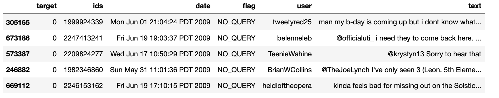
df.sample(5)
Production:
Paso 3: Exploratory data analysis
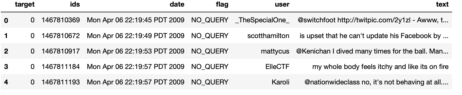
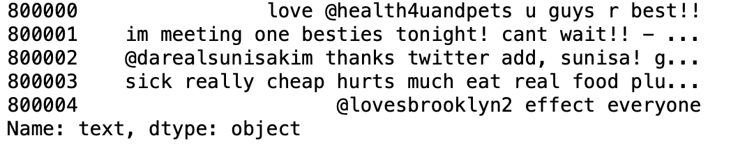
3.1: Five main data registers
df.head()
Production:
3.2: Columns / characteristics in the data
df.columns
Production:
Index(['target', 'ids', 'date', 'flag', 'user', 'text'], dtype="object")
3.3: Data set length
print('length of data is', len(df))
Production:
length of data is 1048576
3.4: Data form
df. shape
Production:
(1048576, 6)
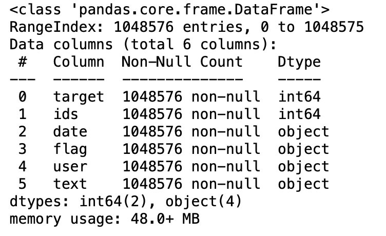
3.5: Data information
df.info()
Production:
3.6: Data types of all columns
df.dtypes
Production:
target     int64
ids        int64
date      object
flag      object
user      object
text      object
dtype: object
3.7: Null value check
np.sum(df.isnull().any(axis=1))
Production:
0
3.8: Rows and columns in the dataset
print('Count of columns in the data is:  ', len(df.columns))
print('Count of rows in the data is:  ', len(df))
Production:
Count of columns in the data is:   6
Count of rows in the data is:   1048576
3.9: Check single objective values
df['target'].unique()
Production:
array([0, 4], dtype=int64)
3.10: Check the number of target values
df['target'].nuniquam()
Production:
2
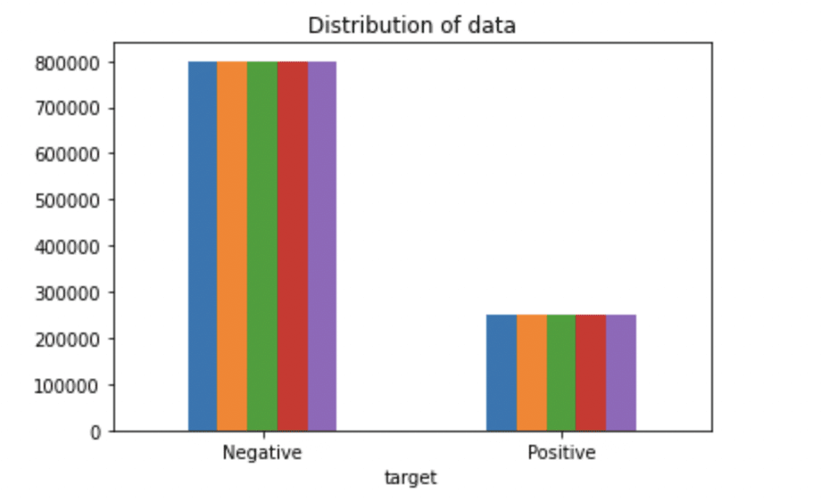
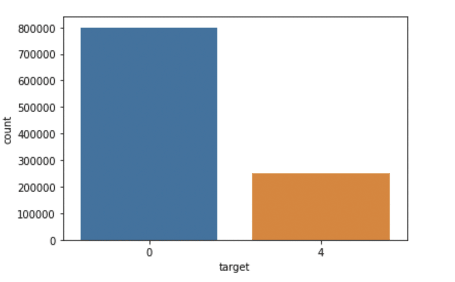
Paso 4: Viewing Target Variable Data
# Plotting the distribution for dataset.
ax = df.groupby('target').count().plot(kind='bar', title="Distribution of data",legend=False)
ax.set_xticklabels(['Negative','Positive'], rotation=0)
# Storing data in lists.
text, sentiment = list(df['text']), list(df['target'])
Production:
import seaborn as sns
sns.countplot(x='target', data=df)
Production:
Paso 5: data preprocessing
In the above problem statement before training the model, we have done several preprocessing steps on the dataset that mainly dealt with removing stopwords, delete emojis. Later, text document is converted to lowercase for better generalization.
Subsequently, scores were cleaned up and removed, thus reducing unnecessary noise from the data set. Thereafter, we have also removed the repeating characters from the words along with removing the urls, since they do not have any significant importance.
Finally, We perform Stemming (reducing words to their derived roots) Y Lematización (reducing derived words to their root form known as a lemma) for best results.
5.1: Select the target text and column for our further analysis
data=df[['text','target']]
5.2: Replacement of values for easier understanding. (Assigning 1 to the positive feeling 4)
data['target'] = data['target'].replace(4,1)
5.3: Print Unique Values of Target Variables
data['target'].unique()
Production:
array([0, 1], dtype=int64)
5.4: Separation of positive and negative tweets
data_pos = data[data['target'] == 1]
data_neg = data[data['target'] == 0]
5.5: taking a quarter of data so that we can run on our machine easily
data_pos = data_pos.iloc[:int(20000)]
data_neg = data_neg.iloc[:int(20000)]
5.6: Combining positive and negative tweets
dataset = pd.concat([data_pos, data_neg])
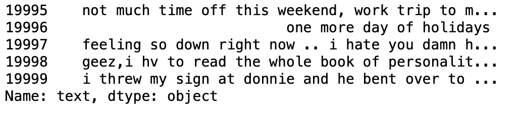
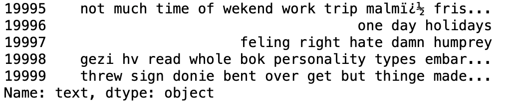
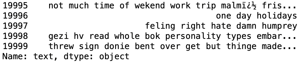
5.7: Make the declaration text lowercase
dataset['text']=dataset['text'].str.lower()
dataset['text'].tail()
Production:
5.8: Definition set containing all stop words in English.
stopwordlist = ['a', 'about', 'above', 'after', 'again', 'ain', 'all', 'am', 'an',
             'and','any','are', 'as', 'at', 'be', 'because', 'been', 'before',
             'being', 'below', 'between','both', 'by', 'can', 'd', 'did', 'do',
             'does', 'doing', 'down', 'during', 'each','few', 'for', 'from',
             'further', 'had', 'has', 'have', 'having', 'he', 'her', 'here',
             'hers', 'herself', 'him', 'himself', 'his', 'how', 'i', 'if', 'in',
             'into','is', 'it', 'its', 'itself', 'just', 'll', 'm', 'ma',
             'me', 'more', 'most','my', 'myself', 'now', 'O', 'of', 'on', 'once',
             'only', 'or', 'other', 'our', 'ours','ourselves', 'out', 'own', 're','s', 'same', 'she', "shes", 'should', "shouldve",'so', 'some', 'such',
             't', 'than', 'that', "thatll", 'the', 'their', 'theirs', 'them',
             'themselves', 'then', 'there', 'these', 'they', 'this', 'those',
             'through', 'to', 'too','under', 'until', 'up', 'and', 'very', 'was',
             'we', 'were', 'what', 'when', 'where','which','while', 'who', 'whom',
             'why', 'will', 'with', 'won', 'and', 'you', "youd","youll", "youre",
             "youve", 'your', 'yours', 'yourself', 'yourselves']
5.9: Clean and remove previous stopword list from tweet text
STOPWORDS = set(stopwordlist)
def cleaning_stopwords(text):
return " ".join([word for word in str(text).split() if word not in STOPWORDS])
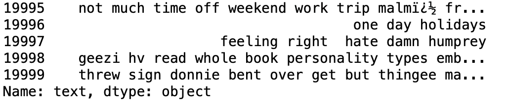
dataset['text'] = dataset['text'].apply(lambda text: cleaning_stopwords(text))
dataset['text'].head()
Production:
5.10: Cleaning and removing scores
import string
english_punctuations = string.punctuation
punctuations_list = english_punctuations
def cleaning_punctuations(text):
    translator = str.maketrans('', '', punctuations_list)
    return text.translate(translator)
dataset['text']= dataset['text'].apply(lambda x: cleaning_punctuations(x))
dataset['text'].tail()
Production:
5.11: Cleaning and removing repeating characters
def cleaning_repeating_char(text):
    return re.sub(r'(.)1+', r'1', text)
dataset['text'] = dataset['text'].apply(lambda x: cleaning_repeating_char(x))
dataset['text'].tail()
Production:

5.12: URL cleaning and removal
def cleaning_URLs(data):
    return re.sub('((www.[^s]+)|(https?://[^s]+))',' ',data)
dataset['text'] = dataset['text'].apply(lambda x: cleaning_URLs(x))
dataset['text'].tail()
Production:
5.13: Cleaning and removing numeric numbers
def cleaning_numbers(data):
    return re.sub('[0-9]+', '', data)
dataset['text'] = dataset['text'].apply(lambda x: cleaning_numbers(x))
dataset['text'].tail()
Production:
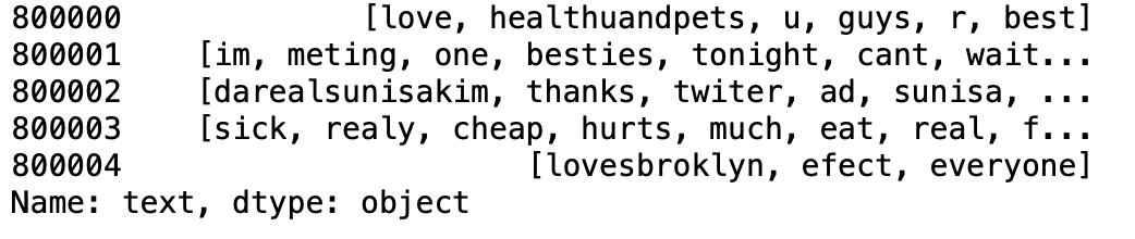
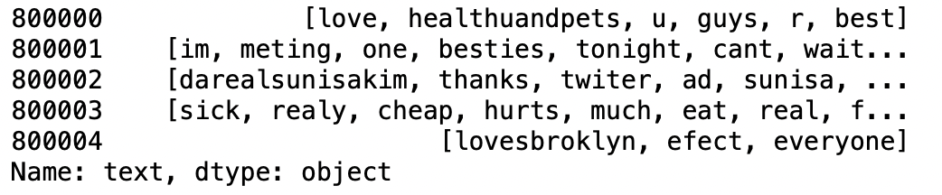
5.14: Obtaining tokenization of the tweet text
from nltk.tokenize import RegexpTokenizer
tokenizer = RegexpTokenizer(r'w+')
dataset['text'] = dataset['text'].apply(tokenizer.tokenize)
dataset['text'].head()
Production:
5.15: Bypass application
import nltk
st = nltk.PorterStemmer()
def stemming_on_text(data):
    text = [st.stem(word) for word in data]
    return data
dataset['text']= dataset['text'].apply(lambda x: stemming_on_text(x))
dataset['text'].head()
Production:
5.16: Lemmatizer application
lm = nltk.WordNetLemmatizer()
def lemmatizer_on_text(data):
    text = [lm.lemmatize(word) for word in data]
    return data
dataset['text'] = dataset['text'].apply(lambda x: lemmatizer_on_text(x))
dataset['text'].head()
Production:
5.17: Separation of input function and label
X=data.text
y=data.target
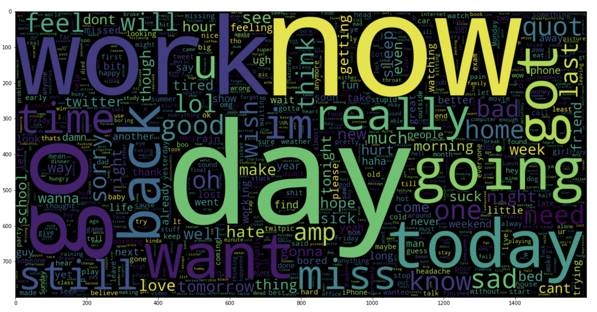
5.18: plot a word cloud for negative tweets
data_neg = data['text'][:800000]
plt.figure(figsize = (20,20))
wc = WordCloud(max_words = 1000 , width = 1600 , height = 800,
               collocations=False).generate(" ".join(data_neg))
plt.imshow(wc)
Production:
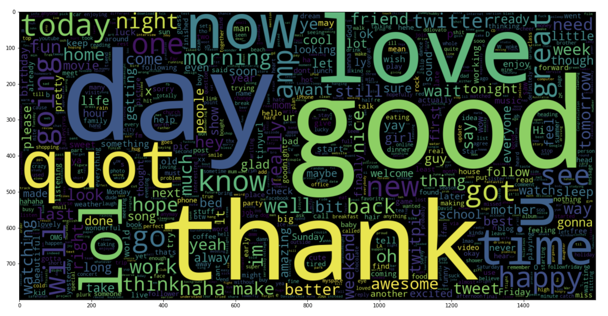
5.19: plot a word cloud for positive tweets
data_pos = data['text'][800000:]
wc = WordCloud(max_words = 1000 , width = 1600 , height = 800,
              collocations=False).generate(" ".join(data_pos))
plt.figure(figsize = (20,20))
plt.imshow(wc)
Production:
Paso 6: Divide our data into training and testing subsets
# Separating the 95% data for training data and 5% for testing data
X_train, X_test, y_train, y_test = train_test_split(X,Y,test_size = 0.05, random_state =26105111)
Paso 7: Transform the dataset using TF-IDF Vectorizer
7.1: Install TF-IDF Vectorizer
vectoriser = TfidfVectorizer(ngram_range=(1,2), max_features=500000)
vectoriser.fit(X_train)
print('No. of feature_words: ', len(vectoriser.get_feature_names()))
Production:
No. of feature_words: 500000
7.2: Transform the data using TF-IDF Vectorizer
X_train = vectoriser.transform(X_train)
X_test  = vectoriser.transform(X_test)
Paso 8: Function for model evaluation
After training the model, we apply the evaluation measures to check the performance of the model. Consequently, We use the following evaluation parameters to verify the performance of the models respectively:
- Accuracy score
- Weft confusion matrix
- Curva ROC-AUC
def model_Evaluate(model):
# Predict values for Test dataset
y_pred = model.predict(X_test)
# Print the evaluation metrics for the dataset.
print(classification_report(y_test, y_pred))
# Compute and plot the Confusion matrix
cf_matrix = confusion_matrix(y_test, y_pred)
categories = ['Negative','Positive']
group_names = ['True Neg','False Pos', 'False Neg','True Pos']
group_percentages = ['{0:.2%}'.format(value) for value in cf_matrix.flatten() / np.sum(cf_matrix)]
labels = [f'{v1}n{v2}' for v1, v2 in zip(group_names,group_percentages)]
labels = np.asarray(labels).reshape(2,2)
sns.heatmap(cf_matrix, annot = labels, cmap = 'Blues',fmt="",
xticklabels = categories, yticklabels = categories)
plt.xlabel("Predicted values", fontdict = {'size':14}, label path = 10)
plt.ylabel("Actual values" , fontdict = {'size':14}, label path = 10)
plt.title ("Confusion Matrix", fontdict = {'size':18}, pad = 20)
Paso 9: Model building
In the statement of the problem we have used three different models respectively:
- Bernoulli ingenuo Bayes
- SVM (support vector machine)
- Logistic regression
The idea behind choosing these models is that we want to test all the classifiers in the dataset, from simple to complex models, and then try to find the one that offers the best performance among them.
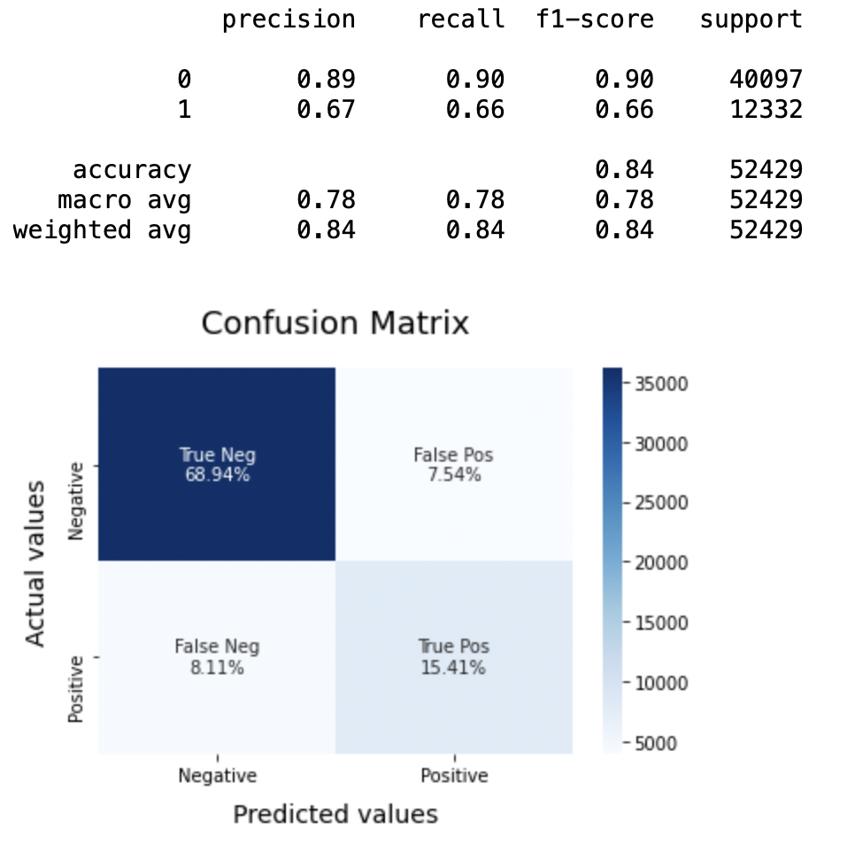
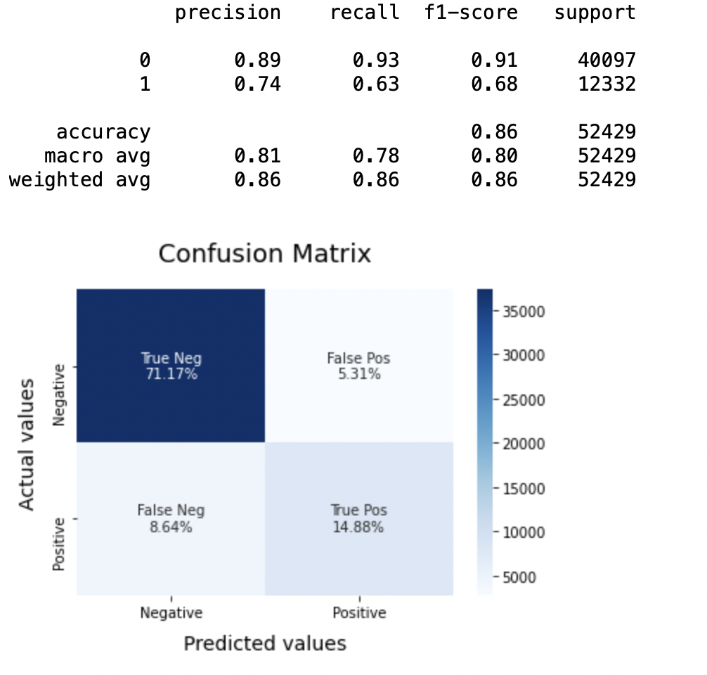
8.1: Model 1
BNBmodel = BernoulliNB()
BNBmodel.fit(X_train, y_train)
model_Evaluate(BNBmodel)
y_pred1 = BNBmodel.predict(X_test)
Production:
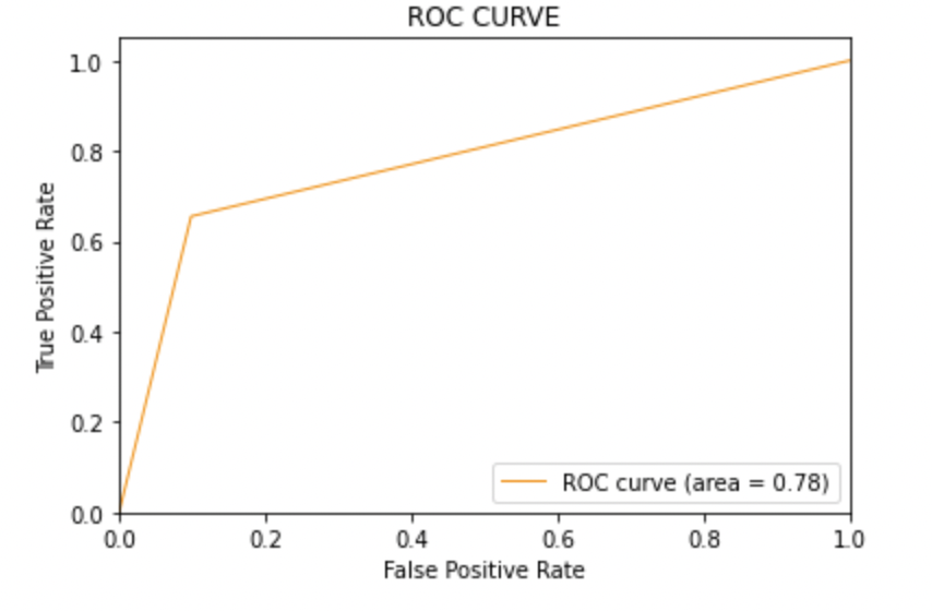
8.2: Plot the ROC-AUC curve for the model 1
from sklearn.metrics import roc_curve, auc
fpr, tpr, thresholds = roc_curve(y_test, y_pred1)
roc_auc = auc(fpr, tpr)
plt.figure()
plt.plot(fpr, tpr, color="darkorange", lw=1, label="ROC curve (area = %0.2f)" % roc_auc)
plt.xlim([0.0, 1.0])
plt.ylim([0.0, 1.05])
plt.xlabel('False Positive Rate')
plt.ylabel('True Positive Rate')
plt.title('ROC CURVE')
plt.legend(loc ="lower right")
plt.show()
Production:
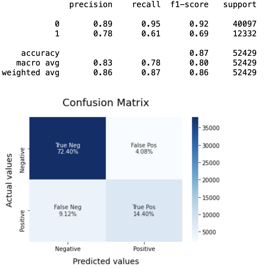
8.3: Model-2:
SVCmodel = LinearSVC()
SVCmodel.fit(X_train, y_train)
model_Evaluate(SVCmodel)
y_pred2 = SVCmodel.predict(X_test)
Production:
8.4: Plot the ROC-AUC curve for the model 2
from sklearn.metrics import roc_curve, auc
fpr, tpr, thresholds = roc_curve(y_test, y_pred2)
roc_auc = auc(fpr, tpr)
plt.figure()
plt.plot(fpr, tpr, color="darkorange", lw=1, label="ROC curve (area = %0.2f)" % roc_auc)
plt.xlim([0.0, 1.0])
plt.ylim([0.0, 1.05])
plt.xlabel('False Positive Rate')
plt.ylabel('True Positive Rate')
plt.title('ROC CURVE')
plt.legend(loc ="lower right")
plt.show()
Production:

8.5: Model-3
LRmodel = LogisticRegression(C = 2, max_iter = 1000, n_jobs=-1)
LRmodel.fit(X_train, y_train)
model_Evaluate(LRmodel)
y_pred3 = LRmodel.predict(X_test)
Production:
8.6: Plot the ROC-AUC curve for the model 3
from sklearn.metrics import roc_curve, auc
fpr, tpr, thresholds = roc_curve(y_test, y_pred3)
roc_auc = auc(fpr, tpr)
plt.figure()
plt.plot(fpr, tpr, color="darkorange", lw=1, label="ROC curve (area = %0.2f)" % roc_auc)
plt.xlim([0.0, 1.0])
plt.ylim([0.0, 1.05])
plt.xlabel('False Positive Rate')
plt.ylabel('True Positive Rate')
plt.title('ROC CURVE')
plt.legend(loc ="lower right")
plt.show()
Production:

Paso 10: Conclution
When evaluating all the models we can conclude the following details, that is,
Precision: Regarding the accuracy of the model, logistic regression works better than SVM, which in turn works better than Bernoulli Naive Bayes.
F1 score: F1 scores for the class 0 and the class 1 son:
(a) For the class 0: Bernoulli Naive Bayes (precision = 0,90) <SVM (precision = 0,91) <Logistic regression (precision = 0,92)
(b) For the class 1: Bernoulli Naive Bayes (precision = 0,66) <SVM (precision = 0,68) <Logistic regression (precision = 0,69)
AUC score: All three models have the same ROC-AUC score.
Therefore, we conclude that logistic regression is the best model for the above data set.
In our problem statement, Logistic regression is following the principle of Occam's Razor which defines that for a particular problem statement, if the data has no assumptions, so the simplest model works best. Since our dataset has no assumptions and the Logistic Regression is a simple model, the concept is valid for the dataset mentioned above.
Final notes
Hope you enjoyed the article.
If you want to connect with me, Do not doubt to keep in touch with me. about Email
Your suggestions and doubts are welcome here in the comments section. Thanks for reading my article!
The media shown in this article is not the property of Analytics Vidhya and is used at the author's discretion.


