What is deep learning? Deep Learning Tutorial

This article was published as part of the Data Science Blogathon.

The guide is mainly for beginners, and I will try to define and emphasize the themes as much as I can. Since deep learning is a very big topic, I would divide the whole tutorial into a few parts. Be sure to read the other parts if you find this helpful.

Contents

1. Introduction

• What is deep learning?
• Why Deep Learning?
• How much data is large?
• Fields where deep learning is used
• Diferencia entre Deep Learning y Machine Learning

2) Import the required libraries

3) Summary

4) Logistic regression

• Computational graph
• Initializing parameters
• Forward propagation
• Optimization with Gradient Descent

5) Logistic regression with Sklearn

6) Final notes

Introduction

What is deep learning?

• It is a subfield of machine learning, inspired by the biological neurons of the brain and translating it into artificial neural networks with representation learning.

Why deep learning?

• When data volume increases, machine learning techniques, no matter how optimized they are, start to become inefficient in terms of performance and accuracy, while deep learning works much better in such cases.

How much data is large?

• Good, a threshold cannot be quantified for the data to be considered large, but, intuitively, Let's say a sample of a million might be enough to say “Is big” (this is where Michael Scott would have pronounced his famous words “That's what she said”).

Fields where DL is used

• Image classification, speech recognition, PNL (natural language processing), recommendation systems, etc.

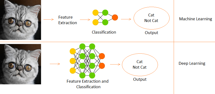
Difference between deep learning and machine learning

• Deep learning is a subset of machine learning.
• En Machine Learning, functions are provided manually.
• While Deep Learning learns functions directly from data.

We will use the Data set of digits in sign language which is available on Kaggle here. Now let's get started.

Import required libraries

import numpy as np # linear algebra
import pandas as pd # data processing, CSV file I / O (e.g. pd.read_csv)
import matplotlib.pyplot as plt
# Input data files are available in the "../input/" directory.
# import warnings
import warnings
# filter warnings
warnings.filterwarnings('ignore')
from subprocess import check_output
print(check_output(["ls", "../input"]).decode("utf8"))
# Any results you write to the current directory are saved as output.

Summary of the data

• There is 2062 images of sign language digits in this dataset.
• Since there is 10 digits of 0 al 9, there is 10 unique signal images.
• In the beginning, we will only use 0 Y 1 (to keep it simple for students)
• In the data, the hand sign for 0 is between the indexes 204 Y 408. There is 205 samples for 0.
• What's more, the hand sign for 1 is between the indexes 822 Y 1027. There is 206 samples.
• Therefore, we will use 205 samples of each class (Note: in reality, 205 samples are much less for a proper deep learning model, but since it is a tutorial, we can ignore it),

Now we will prepare our X and Y matrices, where X is our image matrix (features) and Y is our matrix of labels (0 Y 1).

# load data set
x_l = np.load('../input/Sign-language-digits-dataset/X.npy')
Y_l = np.load('../input/Sign-language-digits-dataset/Y.npy')
img_size = 64
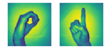
plt.subplot(1, 2, 1)
plt.imshow(x_l[260].reshape(img_size, img_size))
plt.axis('off')
plt.subplot(1, 2, 2)
plt.imshow(x_l[900].reshape(img_size, img_size))
plt.axis('off')

# Join a sequence of arrays along an row axis.
# from 0 to 204 is zero sign and from 205 to 410 is one sign
X = np.concatenate((x_l[204:409], x_l[822:1027] ), axis=0)
z = np.zeros(205)
o = np.ones(205)
Y = np.concatenate((With, O), axis=0).reshape(X.shape[0],1)
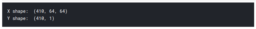
print("X shape: " , X.shape)
print("Y shape: " , Y.shape)

To create our matrix X, We first split and concatenate our segments of hand sign images from 0 Y 1 from data set to matrix X. Then, we do something similar with Y, but we use the tags instead.

1) So we see that the shape of our matrix X is (410, 64, 64)

• The 410 it means 205 images of 0, 205 images of 1.
• the 64 means that the size of our images is 64 x 64 pixels.

2) The Y shape is (410,1), Thus, 410 ones and zeros.

3) Now we divide X and Y into trains and test sets.

• train = 75%, train = 15%
• random_state = Use a particular seed while randomizing, Thus, if the cell runs multiple times, the generated random number does not change every time. The same test and train layout is created each time.

# Then lets create x_train, y_train, x_test, y_test arrays
from sklearn.model_selection import train_test_split
X_train, X_test, Y_train, Y_test = train_test_split(X, Y, test_size=0.15, random_state=42)
number_of_train = X_train.shape[0]
number_of_test = X_test.shape[0]

We have a three-dimensional input matrix, so we have to flatten it to 2D to feed our first deep learning model. As and is already 2D, we leave it as is.

X_train_flatten = X_train.reshape(number_of_train,X_train.shape[1]*X_train.shape[2])
X_test_flatten = X_test .reshape(number_of_test,X_test.shape[1]*X_test.shape[2])
print("X train flatten",X_train_flatten.shape)
print("X test flatten",X_test_flatten.shape)

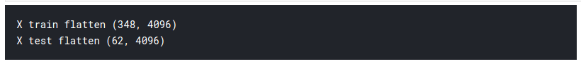
We now have a total of 348 images, each with 4096 pixels in training matrix X. Y 62 images of the same pixel density 4096 in the test matrix. Now we transpose the matrices. This is just a personal choice and you will see in the next codes why I say so.

x_train = X_train_flatten.T
x_test = X_test_flatten.T
y_train = Y_train.T
y_test = Y_test.T
print("x train: ",x_train.shape)
print("x test: ",x_test.shape)
print("there train: ",y_train.shape)
print("y test: ",y_test.shape)

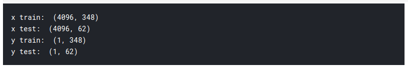
So now we are done with preparing our required data. This is how it looks:

Now we will get acquainted with one of the basic models of Dl, called logistic regression.

Logistic regression

When talking about binary classification, the first model that comes to mind is logistic regression. But one might wonder what is the use of logistic regression in deep learning?? The answer is simple, since logistic regression is a simple neural network. The terms neural network and deep learning go hand in hand. To understand logistic regression, first we have to learn about computer graphics.

Calculation graph

Computer graphics can be considered a pictorial way of representing mathematical expressions. Let's understand that with an example. Suppose we have a simple mathematical expression like:

c = ( a² + b² ) ^1/2

Your computational graph will be:

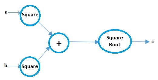
Image source: Author

Now let's look at a logistic regression computational graph:

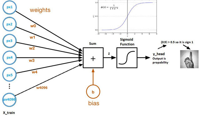
Image source: Kaggle dataset

• The weights and bias are called model parameters.
• The weights represent the coefficients of each pixel.
• The skew is the intersection of the curve formed by plotting parameters against labels.
• Z = (px1 * wx1) + (px2 * wx2) +…. + (px4096 * wx4096)
• y_head = sigmoid_funtion (WITH)
• What the sigmoid function does is essentially scale the value of Z between 0 Y 1, so it becomes a probability.

Why use the sigmoid function?

• It gives us a probabilistic result.
• Since it is a derivative, we can use it in the gradient descent algorithm.

Now we will examine in detail each of the components of the above computational graph.

Initialization parameters

Image source: Microsoft documents

Each pixel has its own weight. But the question is what will your initial weights be? There are several techniques for doing that which I will cover in the part 2 of this article, But for now, we can initialize them using any random value, Let's say 0.01.

The shape of the weight matrix will be (4096, 1), since there is a total of 4096 pixels per image, and let the initial bias be 0.

# lets initialize parameters
# So what we need is dimension 4096 that is number of pixels as a parameter for our initialize method(def)
def initialize_weights_and_bias(dimension):
    w = np.full((dimension,1),0.01)
    b = 0.0
    return w, b

w,b = initialize_weights_and_bias(4096)

Forward propagation

All the steps from the pixels to the cost function are called forward propagation.

To calculate Z we use the formula: Z = (wT) x + b. where x is the pixel matrix, w weights and b is the bias. After calculating Z, we introduce it in the sigmoid function that returns y_head (probability). Thereafter, we calculate the loss function (error).

The cost function is the sum of all losses and penalizes the model for incorrect predictions. This is how our model learns the parameters.

# calculation of z
#z = np.dot(w.T,x_train)+b
def sigmoid(With):
    y_head = 1/(1+np.exp(-With))
    return y_head

y_head = sigmoid(0)
y_head
> 0.5

The mathematical expression of the loss function (log) it is:

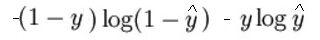
As I said before, what the loss function essentially does is penalize incorrect predictions. here is the code for forward propagation:

# Forward propagation steps:
# find z = w.T*x+b
# y_head = sigmoid(With)
# loss(error) = loss(Y,y_head)
# cost = sum(loss)
def forward_propagation(w,b,x_train,y_train):
    z = e.g. to(w.T,x_train) + b
    y_head = sigmoid(With) # probabilistic 0-1
    loss = -y_train*np.log(y_head)-(1-y_train)*np.log(1-y_head)
    cost = (np.sum(loss))/x_train.shape[1]      # x_train.shape[1]  is for scaling
    return cost

Optimization with Gradient Descent

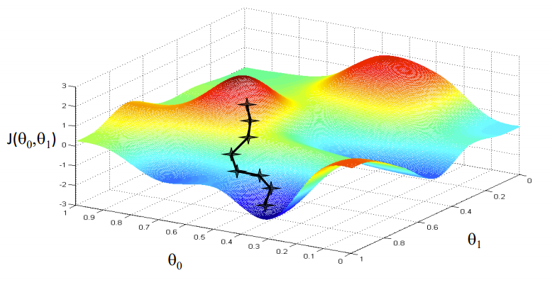
Image source: Coursera

Our goal is to find the values ​​of our parameters for which, the loss function is the minimum. The equation for gradient descent is:

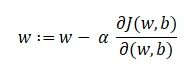
Where w is the weight or the parameter. The Greek letter alpha is something called step size. What it means is the size of the iterations that we will take as we go down the slope to find the local minima. And the remainder is the derivative of the loss function, also known as gradient. The algorithm for gradient descent is simple:

1. First, we take a random data point on our graph and find its slope.
2. Then we find the direction in which the loss function decreases.
3. Update the weights using the above formula. (This method is also called backpropagation.)
4. Select the next point taking a size of α.
5. Repeat.

# In backward propagation we will use y_head that found in forward progation
# Therefore instead of writing backward propagation method, lets combine forward propagation and backward propagation
def forward_backward_propagation(w,b,x_train,y_train):
    # forward propagation
    z = np.dot(w.T,x_train) + b
    y_head = sigmoid(With)
    loss = -y_train*np.log(y_head)-(1-y_train)*np.log(1-y_head)
    cost = (np.sum(loss))/x_train.shape[1]      # x_train.shape[1]  is for scaling
    # backward propagation
    derivative_weight = (np.dot(x_train,((y_head-y_train).T)))/x_train.shape[1] # x_train.shape[1]  is for scaling
    derivative_bias = np.sum(y_head-y_train)/x_train.shape[1]                 # x_train.shape[1]  is for scaling
    gradients = {"derivative_weight": derivative_weight,"derivative_bias": derivative_bias}
    return cost,gradients

Now we update the learning parameters:

# Updating(learning) parameters
def update(w, b, x_train, y_train, learning_rate,number_of_iterarion):
    cost_list = []
    cost_list2 = []
    index = []
    # updating(learning) parameters is number_of_iterarion times
    for i in range(number_of_iterarion):
        # make forward and backward propagation and find cost and gradients
        cost,gradients = forward_backward_propagation(w,b,x_train,y_train)
        cost_list.append(cost)
        # lets update
        w = w - learning_rate * gradients["derivative_weight"]
        b = b - learning_rate * gradients["derivative_bias"]
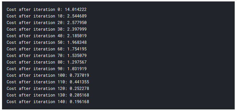
        if i % 10 == 0:
            cost_list2.append(cost)
            index.append(i)
            print ("Cost after iteration %i: %f" %(i, cost))
    # we update(learn) parameters weights and bias
    parameters = {"weight": w,"bias": b}
    plt.plot(index,cost_list2)
    plt.xticks(index,rotation='vertical')
    plt.xlabel("Number of Iterarion")
    plt.ylabel("Cost")
    plt.show()
    return parameters, gradients, cost_list

parameters, gradients, cost_list = update(w, b, x_train, y_train, learning_rate = 0.009,number_of_iterarion = 200)

So far, we learned our parameters. It means that we are adjusting the data. In the prediction step, we have x_test as input and using it, we make forward predictions.

 # prediction
def predict(w,b,x_test):
    # x_test is a input for forward propagation
    z = sigmoid(np.dot(w.T,x_test)+b)
    Y_prediction = np.zeros((1,x_test.shape[1]))
    # if z is bigger than 0.5, our prediction is sign one (y_head=1),
    # if z is smaller than 0.5, our prediction is sign zero (y_head=0),
    for i in range(z.shape[1]):
        if z[0,i]<= 0.5:
            Y_prediction[0,i] = 0
        else:
            Y_prediction[0,i] = 1

    return Y_prediction

predict(parameters["weight"],parameters["bias"],x_test)

Now we make our predictions. Let's put it all together:

def logistic_regression(x_train, y_train, x_test, y_test, learning_rate ,  num_iterations):
    # initialize
    dimension =  x_train.shape[0]  # that is 4096
    w,b = initialize_weights_and_bias(dimension)
    # do not change learning rate
    parameters, gradients, cost_list = update(w, b, x_train, y_train, learning_rate,num_iterations)
    
    y_prediction_test = predict(parameters["weight"],parameters["bias"],x_test)
    y_prediction_train = predict(parameters["weight"],parameters["bias"],x_train)

    # Print train/test Errors
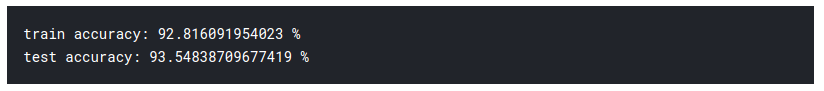
    print("train accuracy: {} %".format(100 - np.mean(np.abs(y_prediction_train - y_train)) * 100))
    print("test accuracy: {} %".format(100 - np.mean(np.abs(y_prediction_test - y_test)) * 100))
    
logistic_regression(x_train, y_train, x_test, y_test,learning_rate = 0.01, num_iterations = 150)

Then, as you can see, even the most fundamental model of deep learning is quite difficult. It is not easy for you to learn, and beginners can sometimes feel overwhelmed studying all of this at once. But the thing is, we haven't touched deep learning yet., this is like the surface. There is much more that I will add in the part 2 of this article.

Since we have learned the logic behind logistic regression, we can use a library called SKlearn which already has many of the built-in models and algorithms, so you don't have to start everything from scratch.

Logistic regression with Sklearn

I'm not going to explain much in this section since you know almost all the logic and intuition behind logistic regression.. If you are interested in reading about the Sklearn library, you can read the official documentation here. Here is the code, and I'm sure you'll be stunned to see how little effort it takes:

from sklearn import linear_model
logreg = linear_model.LogisticRegression(random_state = 42,max_iter= 150)
print("test accuracy: {} ".format(logreg.fit(x_train.T, y_train.T).score(x_test.T, y_test.T)))
print("train accuracy: {} ".format(logreg.fit(x_train.T, y_train.T).score(x_train.T, y_train.T)))

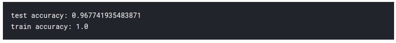
Yes! this is all it took, ¡solo 1 line of code!

Final notes

We have learned a lot today. But this is only the beginning. Be sure to check out the part 2 of this article. You can find it in the following link. If you like what you read, you can read some of the other interesting articles I have written.

Sion | Author at DataPeaker

I hope you had a good time reading my article. Health!!

Media shown in this article about top machine learning libraries in Julia is not the property of DataPeaker and is used at the author's discretion.

Related