keep in mind javascript is required for full website functionality.

Welcome back to our regular blog of Excel functions from A to Z. Today we look at the DOLLAR function.
The DOLLAR function
This function converts a number to text format and apply a currency symbol. The name of the function (and the symbol that applies) depends on language setting. For instance, with our Australian configuration, this function converts a number to text in currency format, with decimals rounded to the specified place. The format used is $ #, ## 0.00 _); ($ #, ## 0.00). For more information on the custom number format, see link here.
The DOLLAR The function uses the following syntax to operate:
DOLLAR (number, [decimals])
The DOLLAR The function has the following arguments:
- number: this is necessary and represents a number, a reference to a cell that contains a number or a formula that evaluates to number
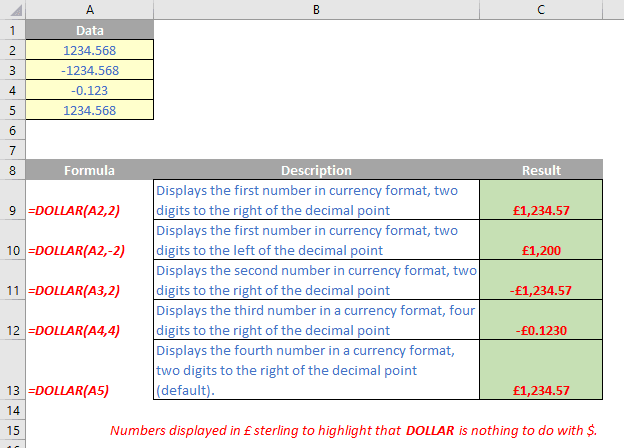
- decimals: this argument is optional. This denotes the number of digits to the right of the decimal point. And decimals is a negative value, number is rounded to the left of the decimal point. If you omit decimals, it's supposed to be two (2).
It should also be noted that the difference between formatting a cell with a ribbon command and using the DOLLAR function is that DOLLAR converts its result to text. A number formatted with the ‘Format Cells dialog box’ (CTRL + 1) still a number. Microsoft claims that you can continue to use the results generated by DOLLAR in other formulas, because Excel converts numbers entered as text to numbers when calculating. But nevertheless, that's not true, since the following [UK] example shows:
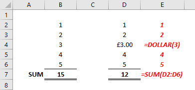
Please, see my example below:
Soon we will continue with our functions from A to Z of Excel. Keep checking: there is a new blog post every business day.
You can find a full page of feature articles here.


