Introduction:
In this article, we will learn all the important statistical concepts that are required for data science roles.
Table of Contents:
- Difference between parameter and statistic
- Statistics and their types
- Data types and measurement levels
- Business decision moments
- Central limit theorem (CLT)
- Probability distributions
- Graphical representations
- Hypothesis testing
1. Difference between parameter and statistic
In our day to day we continue talking about Population and shows. Then, it is very important to know the terminology to represent the population and the sample.
A parameter is a number that describes the population data. And a statistic is a number that describes the data in a sample.
2. Statistics and their types
The Wikipedia definition of Statistics states that “is a discipline that deals with the compilation, organization, analysis, interpretation and presentation of data”.
Means that, as part of the statistical analysis, we collect, organize and extract meaningful information from data, either through visualizations or mathematical explanations.
Statistics are broadly classified into two types:
- Descriptive statistics
- Inferential statistics
Descriptive statistics:
As the name suggests in Descriptive Statistics, We describe the data using the Mean distributions, Standard deviation, Graphs or Probability.
Basically, as part of the descriptive statistics, we measure the following:
- Frequency: no. number of times a data point occurs
- Central trend: the centrality of data: media, medianThe median is a statistical measure that represents the central value of a set of ordered data. To calculate it, the data is organized from lowest to highest and the number in the middle is identified. If there are an even number of observations, the two core values are averaged. This indicator is especially useful in asymmetric distributions, since it is not affected by extreme values.... and fashion.
- Dispersion: the extent of the data: rank, variance and standard deviation
- The measureThe "measure" it is a fundamental concept in various disciplines, which refers to the process of quantifying characteristics or magnitudes of objects, phenomena or situations. In mathematics, Used to determine lengths, Areas and volumes, while in social sciences it can refer to the evaluation of qualitative and quantitative variables. Measurement accuracy is crucial to obtain reliable and valid results in any research or practical application.... of the position: percentiles and quantile ranges
Inferential statistics:
In Inferential Statistics, estimamos los parametersThe "parameters" are variables or criteria that are used to define, measure or evaluate a phenomenon or system. In various fields such as statistics, Computer Science and Scientific Research, Parameters are critical to establishing norms and standards that guide data analysis and interpretation. Their proper selection and handling are crucial to obtain accurate and relevant results in any study or project.... de población. Or we perform hypothesis tests to evaluate the assumptions made about the population parameters..
In simple terms, we interpret the meaning of descriptive statistics by inferring them to the population.
For instance, we are conducting a survey on the number of two-wheelers in a city. Suppose the city has a total population of 5L people. Therefore, we take a sample of 1000 people, as it is impossible to perform an analysis of the entire population data.
From the survey carried out, it is found that 800 people from 1000 (800 of 1000 it is 80%) they are two-wheelers. Then, we can infer these results to the population and conclude that the 4L people from the 5L population are two-wheelers.
3. Data types and measurement level
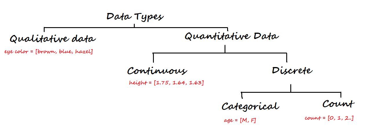
On a higher level, data is classified into two types: Qualitative Y Quantitative.
Qualitative data is not numerical. Some of the examples are eye color, car brand, the city, etc.
Secondly, quantitative data is numerical and again divided into continuous and discrete data.
Continuous data: Can be represented in decimal format. Some examples are height, weight, weather, distance, etc.
Discrete data: Cannot be represented in decimal format. Some examples are the number of laptops, the number of students in a class.
Discrete data is split back into categorical and count data.
Categorical data: represent the type of data that can be divided into groups. Some examples are age, sex, etc.
Count data: These data contain non-negative integers. Example: number of children a partner has.
Measurement level
In statistics, el nivel de medición es una clasificación que describe la relación entre los valores de una variableIn statistics and mathematics, a "variable" is a symbol that represents a value that can change or vary. There are different types of variables, and qualitative, that describe non-numerical characteristics, and quantitative, representing numerical quantities. Variables are fundamental in experiments and studies, since they allow the analysis of relationships and patterns between different elements, facilitating the understanding of complex phenomena.....
We have four fundamental levels of measurement. Son:
- Nominal scale
- Ordinal scale
- Interval scale
- Proportion scale
1. Nominal scale: This scale contains the least amount of information since the data only has names / labels. Can be used for classification. We cannot perform mathematical operations on nominal data because there is no numerical value for the options (the numbers associated with the names can only be used as labels).
Example: To what country do you belong? India, Japan, Korea.
2. Ordinal scale: Compared to the nominal scale, the ordinal scale has more information because together with the labels, has order / address.
Example: Income level: high income, average income, low incomes.
3. Interval scale: It is a numerical scale. The interval scale has more information than the nominal ordinal scales. Along with the order, we know the difference between the two variables (the interval indicates the distance between two entities).
The average can be used, the median and mode to describe the data.
Example: temperature, income, etc.
4. Ratio scale: The ratio scale has the most information about the data. Unlike the other three scales, the ratio scale can accommodate a true zero point. It is simply said that the ratio scale is the combination of scales Nominal, Ordinal e Intercal.
Example: actual weight, height, etc.
4. Business decision moments
We have four business decision moments that help us understand the data.
4.1. Measures of central tendency
(Also known as a business decision in the first place)
Talk about the centrality of data. to simplify it, is part of the descriptive statistical analysis in which a single value in the center represents the entire data set.
The central tendency of a data set can be measured by:
To mean: It is the sum of all data points divided by the total number of values in the data set. The mean cannot always be trusted because it is influenced by outliers.
Median: It is the intermediate value of an ordered data set / tidy. If the size of the data set is even, the median is calculated by taking the average of the two mean values.
Way: It is the most repeated value in the data set. Data with only one mode is called unimodal, data with two modes is called bimodal and data with more than two modes is called multimodal.
4.2. Measures of dispersion
(Also known as a second-time business decision)
Talk about the dissemination of data from your center.
Dispersion can be measured using:
Difference: It is the average squared distance of all data points from its mean. The problem with variance is that the units will also square.
Standard deviation: It is the square root of the variance. Helps to recover original drives.
Distance: It is the difference between the maximum and minimum values of a data set.
Measure |
Population |
Shows |
| To mean | µ = (Σ XI)/NORTH | x̄ = (Σ xI)/North |
| Median | The mean value of the data | The mean value of the data |
| Way | Most occurred value | Most occurred value |
| Difference | σ2 = (Σ XI – µ)2/NORTH | s2 = (Σ xI – X )2/ (n-1) |
| Standard deviation | σ = square root ((Σ XI – µ)2/NORTH) | s = square root ((Σ xI – X )2/ (n-1)) |
| Distance | Maximum minimum | Maximum minimum |
4.3. Obliquity
(It is also known as a business decision in the third moment)
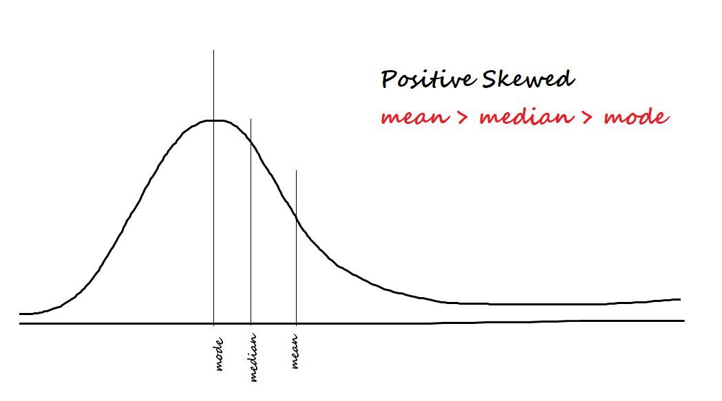
Measure skewness in data. The two types of asymmetry are:
Positive / skewed to the right: The data is said to be positively biased if most of the data is concentrated on the left side and has a tail to the right.
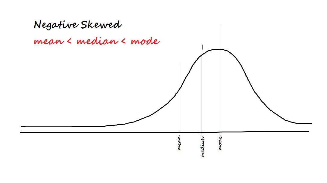
Negative / skewed to the left: The data is said to be negatively biased if most of the data is concentrated on the right side and has a tail to the left.
The asymmetry formula is me [(X - µ)/ σ ]) 3 = Z3
4.4. Curtosis
(Also known as a fourth-moment business decision)
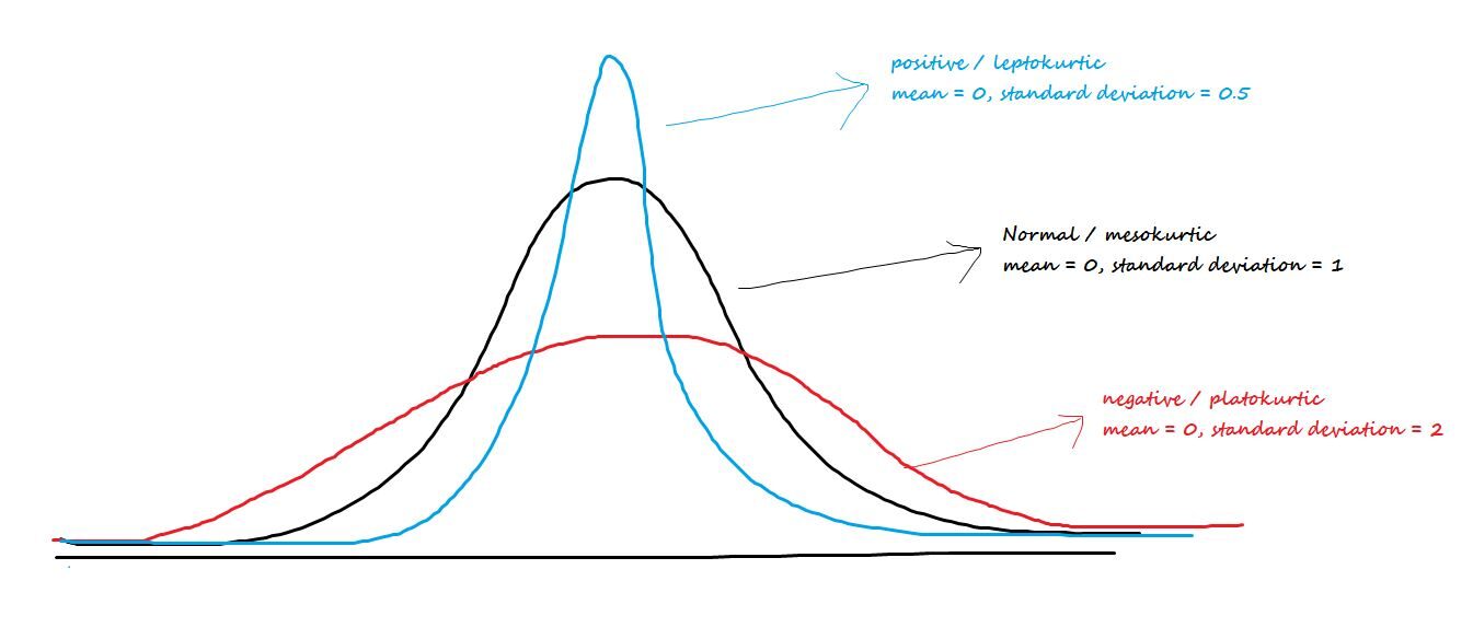
Talk about the central peak or the plumpness of the tails. The three types of kurtosis are:
Positive / leptocurtic: Has sharp beaks and lighter tails.
Negative / Platokúrtico: Has wide beaks and thicker tails.
mesokurtic: Normal distribution
The kurtosis formula is me [(X - µ)/ σ ]) 4-3 = Z4– 3
Together, skewness and kurtosis are called shape statistics.
5. Central limit theorem (CLT)
Instead of analyzing the data of the entire population, we always take a sample for analysis. The problem with sampling is that “the sample mean is a random variable, varies for different samples ". And the random sample we draw can never be an exact representation of the population. This phenomenon is called sample variation.
To cancel the sample variation, we use the central limit theorem. And according to the central limit theorem:
1. The distribution of the sample means follows a normal distribution if the population is normal.
2. the distribution of the sample means follows a normal distribution even though the population is not normal. But the sample size should be large enough.
3. The grand average of all sample mean values gives us the population mean.
4. Theoretically, the sample size should be 30. And practically, the condition about sample size (n) it is:
n> 10 (k3)2, where k3 is the asymmetry of the sample.
n> 10 (k4), where K4 is the kurtosis sample.
6. Probability distributions
In statistical terms, a distribution function is a mathematical expression that describes the probability of different possible outcomes for an experiment.
Please, read this article of mine on the different types of probability distributions.
7. Graphical representations
Graphical representation refers to the use of tables or graphs to visualize, analyze and interpret numerical data.
For a single variable (univariate analysis), we have a bar chart, a line diagram, a frequency diagram, a dot plot, a box plot and the normal QQ plot.
We will discuss the box plot and the normal QQ plot.
7.1. Box plot
A box plot is a way to visualize the distribution of data based on a five-number summary. Used to identify outliers in the data.
The five numbers are minimum, first quartile (Q1), median (Q2), third quartile (Q3) and maximum.
The box region will contain the 50% of the data. The 25% bottom of the data region is called the Bottom Whisker and the bottom 25% top of the data region is called Top Whisker.
The interquartile region (IQR) is the difference between the third and the first quartile. IQR = Q3 – Q1.
Outliers are the data points below the lower whisker and beyond the upper whisker.
The formula for finding outliers is Outlier = Q ± 1,5 * (IQR)
The outliers below the lower whisker are given as Q1 – 1,5 * (IQR)
Outliers beyond the upper whisker are given as Q3 + 1.5 * (IQR)
See my article on detecting outliers using a box plot.
7.2. Normal QQ chart
Un diagrama de QQ normal es una especie de Dispersion diagramThe scatter plot is a graphical tool used in statistics to visualize the relationship between two variables. It consists of a set of points in a Cartesian plane, where each point represents a pair of values corresponding to the variables analyzed. This type of chart allows you to identify patterns, Trends and possible correlations, facilitating data interpretation and decision-making based on the visual information presented.... que se traza creando dos conjuntos de cuantiles. It is used to check whether the data is normal or not.
On the x-axis we have the Z scores and on the y-axis we have the actual sample quantiles. If the scatter plot forms a straight line, the data is said to be normal.
8. Hypothesis testing
Hypothesis testing in statistics is a way of testing assumptions made about population parameters.
See my article on hypothesis testing to read it in detail.
Final notes:
Thanks for reading to the conclusion. At the end of this article, we are familiar with important statistical concepts.
I hope this article is informative. Feel free to share it with your fellow students.
Other blog posts of mine
Feel free to check out my other blog posts from my DataPeaker profile.
You can find me in LinkedIn, Twitter in case you want to connect. I would love to connect with you.
For an immediate exchange of thoughts, write to me [email protected].
The media shown in this article is not the property of DataPeaker and is used at the author's discretion.


