This article was published as part of the Data Science Blogathon
1. Introduction
In this work, presentamos la relación del rendimiento del modelo con un tamaño de conjunto de datos variableIn statistics and mathematics, a "variable" is a symbol that represents a value that can change or vary. There are different types of variables, and qualitative, that describe non-numerical characteristics, and quantitative, representing numerical quantities. Variables are fundamental in experiments and studies, since they allow the analysis of relationships and patterns between different elements, facilitating the understanding of complex phenomena.... y un número variable de clases de destino. We have conducted our experiments on Amazon product reviews.
The dataset contains the title of the review, the review text and ratings. We have considered grades as our exit class. What's more, we have carried out three experiments (polarity 0/1), three classes (positive, negative, neutral) and five classes (rating of 1 a 5). Hemos incluido tres modelos tradicionales y tres de deep learningDeep learning, A subdiscipline of artificial intelligence, relies on artificial neural networks to analyze and process large volumes of data. This technique allows machines to learn patterns and perform complex tasks, such as speech recognition and computer vision. Its ability to continuously improve as more data is provided to it makes it a key tool in various industries, from health....
Machine learning models
1. Logistic regression (LR)
2. Support Vector Machine (SVM)
3. Naive-Bayes (NB)
Deep learning models
1. Red neuronalNeural networks are computational models inspired by the functioning of the human brain. They use structures known as artificial neurons to process and learn from data. These networks are fundamental in the field of artificial intelligence, enabling significant advancements in tasks such as image recognition, Natural Language Processing and Time Series Prediction, among others. Their ability to learn complex patterns makes them powerful tools.. de convolución (CNN)
2. Short term memory (LSTM)
3. Recurring unit closed (CRANE)
2. The data set
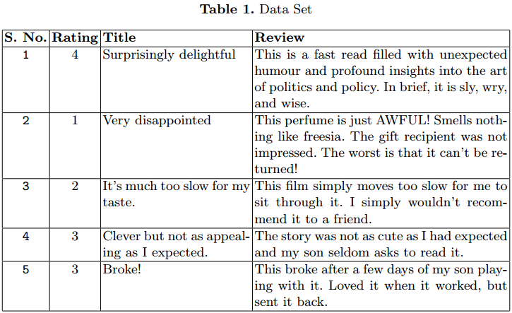
We used Amazon's product review dataset for our experiment. The data set contains 3,6 million instances of the product review in text form.
Separate train files have been provided (3M) and test (0,6M) in CSV format. Each instance has 3 attributes. The first attribute is the classification Come in 1 Y 5. The second attribute is the qualification Of the review. The last one is the revision text.
In the table 1 there are some cases. We have considered only 1,5 M.
3. Experiment for analysis
We have already mentioned that the whole experiment was performed for binary classification, three-class and five-class. We have done some pre-processing steps on the dataset before passing it on to the classification models. Each experiment was performed incrementally.
We start our training with 50000 instances and we increase to 1,5 million instances for training. Finally, registramos los parametersThe "parameters" are variables or criteria that are used to define, measure or evaluate a phenomenon or system. In various fields such as statistics, Computer Science and Scientific Research, Parameters are critical to establishing norms and standards that guide data analysis and interpretation. Their proper selection and handling are crucial to obtain accurate and relevant results in any study or project.... de rendimiento de cada modelo.
3.1 Preprocessing
3.1.1 Label mapping:
We have considered the grades as the class for the revision text. The grade attribute range is between 1 Y 5. We need to assign these grades to the number of classes, considered for the particular experiment.
a) Binary classification: –
Here, we assign the grade 1 Y 2 to the class 0 and rating 4 Y 5 to class 1. This form of classification can be treated as a feeling classification problem., where the reviews with 1 Y 2 grades are in negative class and 4 Y 5 they are in positive class.
We have not considered reviews with a rating of 3 for the binary classification experiment. Therefore, obtenemos menos instancias para el trainingTraining is a systematic process designed to improve skills, physical knowledge or abilities. It is applied in various areas, like sport, Education and professional development. An effective training program includes goal planning, regular practice and evaluation of progress. Adaptation to individual needs and motivation are key factors in achieving successful and sustainable results in any discipline.... en comparación con los otros dos experimentos.
b) Classification of three classes: –
Here, we extend our previous classification experiment. Now we consider the rating 3 as a new separate class. The new assignment of grades to classes is as follows: Qualification 1 Y 2 assigned to class 0 (Negative), Classification 3 assigned to class 1 (Neutral) and rating 4 Y 5 assigned to class 2 (Positive).
Instances for class 1 they are far inferior to the class 0 Y 2, which creates a class imbalance problem. Therefore, we use micropromedio when calculating performance measures.
c) Five-class classification: –
Here, we consider each grade as a separate class. The assignment is as follows: Classification 1 assigned to class 0, Classification 2 assigned to class 1, Classification 3 assigned to class 2, Classification 4 assigned to class 3and the classification 5 assigned to class 4.
3.1.2 Review text pre-processing:
Amazon product reviews are in text format. We need to convert the text data to a numeric format, which can be used to train models.
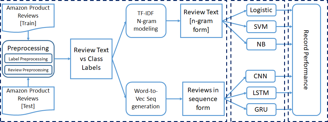
For machine learning models, we convert the revision text into TF-IDF vector format with the help of the sklearn Library. Instead of taking each word individually, we consider the n-gram model while creating the TF IDF vectors. The range of N-grams is set to 2 – 3, and the maximum function value is set to 5000.
For deep learning models, we need to convert the text sequence data to number sequence data. We apply the word to vector modeling to convert each word to the equivalent vector.
The data set contains a large number of words; Thus, hot coding 1- it is very ineffective. Here we have used a pre-trained word2Vec model to represent each word with a column vector of size 300. We set the maximum length of the sequence equal to 70.
Reviews with a word length less than 70 are padded with leading zeros. For reviews with a word length greater than 70, we select the first 70 words for word2Vec processing.
3.2 Classification model training
We mentioned earlier that we have taken three traditional machine learning models (LR, SVM, NB) and three deep learning models (CNN, LSTM, CRANE). Preprocessed text with label information is passed to templates for training.
In the beginning, we train the six models with 50000 instances and we test them with 5000 instances. For the next iteration, we add 50000 Y 5000 more instances in the train and the test set, respectively. We perform 30 iterations; Thus, We consider 1.5 M, 150000 instances for the train and test set in the last iteration.
The training mentioned above is done for all three types of classification experiments..
3.3 Model configurations
We have used the default hyperparameter settings of all the traditional classifiers used in this experiment. And CNN, the input size is 70 with an inlay size of 300. Key layer skip is set to 0.3. A 1-D convolution has been applied to the input, with the convolution output size set to 100. The kernel size is kept at 3. resumeThe ReLU activation function (Rectified Linear Unit) It is widely used in neural networks due to its simplicity and effectiveness. Defined as ( f(x) = max(0, x) ), ReLU allows neurons to fire only when the input is positive, which helps mitigate the problem of gradient fading. Its use has been shown to improve performance in various deep learning tasks, making ReLU an option... The wake functionThe activation function is a key component in neural networks, since it determines the output of a neuron based on its input. Its main purpose is to introduce nonlinearities into the model, allowing you to learn complex patterns in data. There are various activation functions, like the sigmoid, ReLU and tanh, each with particular characteristics that affect the performance of the model in different applications.... se ha utilizado en la capa de convolución. For the grouping process, maximum grouping is used. El Optimizador de Adam se utiliza con una Loss functionThe loss function is a fundamental tool in machine learning that quantifies the discrepancy between model predictions and actual values. Its goal is to guide the training process by minimizing this difference, thus allowing the model to learn more effectively. There are different types of loss functions, such as mean square error and cross-entropy, each one suitable for different tasks and... de entropía cruzada.
LSTM and GRU also have the same hyperparameter settings. El tamaño de la Output layerThe "Output layer" is a concept used in the field of information technology and systems design. It refers to the last layer of a software model or architecture that is responsible for presenting the results to the end user. This layer is crucial for the user experience, since it allows direct interaction with the system and the visualization of processed data.... cambia con el experimento en ejecución.
3.4 Performance measures
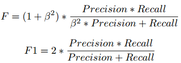
Scoring formula F
We have taken the F1 score to analyze the performance of the classification models with different class labels and instance count. There is a trade-off between Precision and Recall if we try to improve Recall, Precision would be compromised, and the same applies in reverse.
The F1 score combines precision and recall in the form of a harmonic mean.
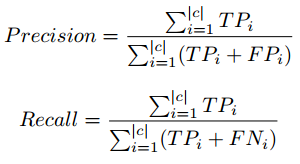
Precision, micro-average recovery formula
In the classification of three and five classes, we observe that the count of instances with qualification 3 is much lower in comparison to other ratings, what creates the class imbalance problem.
Therefore, we use the concept of micro-averaging when calculating performance parameters. Micro-averaging takes care of class imbalance when calculating accuracy and recall. For detailed information on Precision, Recall, visit the following link: enlace wiki.
4 Results and observation
In this section, we have presented the results of our experiments with different sizes of data sets and the number of class labels. A separate graph has been presented for each experiment.. Charts are plotted between test set size and F1 score.
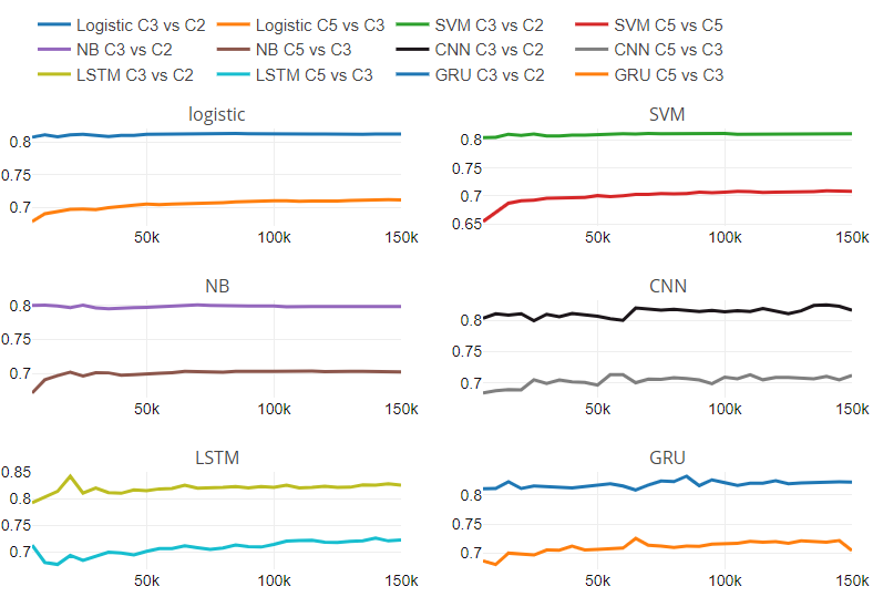
What's more, proporcionamos la Figure"Figure" is a term that is used in various contexts, From art to anatomy. In the artistic field, refers to the representation of human or animal forms in sculptures and paintings. In anatomy, designates the shape and structure of the body. What's more, in mathematics, "figure" it is related to geometric shapes. Its versatility makes it a fundamental concept in multiple disciplines.... 5, containing six subplots. Each subplot corresponds to a classifier. We have presented the rate of change between the performance scores of two experiments with respect to the variable size of the test set.
Figure 2
The figure 2 presents the performance of the classifiers in the binary classification task. In this case, the actual size of the test is smaller than the data we have taken for the test because the rated reviews were removed 3.
Machine learning classifiers (LR, SVM, NB) run consistently except for slight variations in starting points.
The deep learning classifier (GRU and CNN) starts out with less performance compared to SVM and LR. After three initial iterations, GRU and CNN continually dominate machine learning classifiers.
LSTM makes learning more effective. LSTM started with the lowest performance. A measureThe "measure" it is a fundamental concept in various disciplines, which refers to the process of quantifying characteristics or magnitudes of objects, phenomena or situations. In mathematics, Used to determine lengths, Areas and volumes, while in social sciences it can refer to the evaluation of qualitative and quantitative variables. Measurement accuracy is crucial to obtain reliable and valid results in any research or practical application.... que el conjunto de entrenamiento cruza 0.3 M, LSTM has shown continued growth and ended with GRU.
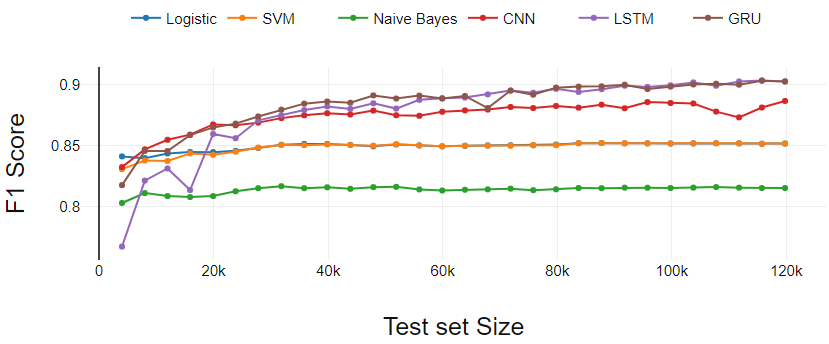
Fig 2. Binary classification performance analysis
figure 3
The figure 3 presents the results of the three-class classification experiment. Performance of all classifiers degrades as classes increase. The performance is similar to binary classification if we compare a particular classifier with others.
The only difference is in the performance of LSTM. Here, LSTM has continuously increased performance unlike binary sorting. LR worked a bit better compared to SVM. Both LR and SVM performed equally in the binary classification experiment..
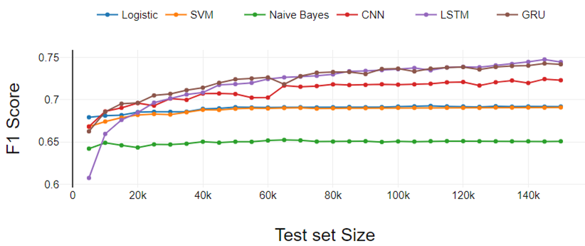
Fig 3. Three-class classification performance analysis
Figure 4
The figure 4 represents the results of the five-class classification experiment. The results follow the same trends that appeared in the binary and three-class classification experiment.. Here the performance difference between LR and SVM increased a bit more.
Therefore, we can conclude that the performance gap of LR and SVM increases as the number of classes increases.
From the general analysis, deep learning classifiers perform better as training dataset size increases and traditional classifiers show consistent performance.
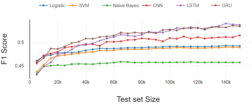
Fig 4. Five-class ranking performance analysis
Figure 5
The figure 5 represents the performance ratio with respect to the change in the number of classes and the size of the data set. The figure contains six subplots, one for each classifier. Each subplot has two lines; one line shows the performance relationship between the three-class classification and the binary class on different sizes of data sets.
Another line represents the performance relationship between the five-class and three-class classification on different sizes of data sets.. We have found that traditional classifiers have a constant rate of change. For traditional classifiers, rate of change is independent of the size of the data set. We cannot comment on the behavior of deep learning models with respect to change in numerical classes and dataset size due to variable pattern in rate of change.
In addition to the experimental analysis mentioned above, we have analyzed misclassified text data. We found interesting observations that affected the classification.
Sarcastic words: –
Customers wrote sarcastic reviews about the products. They have given the rating 1 O 2, but they used a lot of positive polarity words. For instance, a client rated 1 and wrote the following review: “¡Oh! What a fantastic charger I have !! ”. The classifier got confused with these kinds of polarity words and phrases.
Use of high polarity words: –
Clients have given an average rating (3) but they used very polarized words in their reviews. For instance, Fantastic, tremendous, notable, pathetic, etc.
Use of weird words: –
Having a dataset of size 3.6M, we still find many uncommon words, that affected the performance of the classification. Spelling errors, acronyms, short form words used by reviewers are also important factors.
5. Final note
We have analyzed the performance of traditional machine learning and deep learning models with different sizes of data sets and the number of the target class.
We have found that traditional classifiers can learn better than deep learning classifiers if the data set is small.. With the increase in the size of the dataset, deep learning models get a performance boost.
We have investigated the rate of change in the performance of the binary to three classes Y three classes to five classes problem with variable dataset size.
We have used Hard deep learning library for experimentation. Python results and scripts are available at the following link: GitHub link.
The media shown in this article is not the property of DataPeaker and is used at the author's discretion.


