This article was published as part of the Data Science Blogathon
After understanding and working with this practical tutorial, may:
- Understand what cohort and cohort analysis is.
- Handling missing values
- Extraction of the month from the date
- Asignar cohorte a cada transactionThe "transaction" refers to the process by which an exchange of goods takes place, services or money between two or more parties. This concept is fundamental in the economic and legal field, since it involves mutual agreement and consideration of specific terms. Transactions can be formal, as contracts, or informal, and are essential for the functioning of markets and businesses....
- Asignar indexThe "Index" It is a fundamental tool in books and documents, which allows you to quickly locate the desired information. Generally, it is presented at the beginning of a work and organizes the contents in a hierarchical manner, including chapters and sections. Its correct preparation facilitates navigation and improves the understanding of the material, making it an essential resource for both students and professionals in various areas.... de cohorte a cada transacción
- Calculate the number of unique customers in each group.
- Create a cohort table for the retention rate
- Visualice la tabla de cohortes usando el heat mapa "heat map" is a graphical representation that uses colors to show the density of data in a specific area. Commonly used in data analytics, Marketing and behavioral studies, This type of visualization allows you to identify patterns and trends quickly. Through chromatic variations, Heat maps make it easier to interpret large volumes of information, helping to make informed decisions....
- Interpret the retention rate
What is cohort and cohort analysis?
A cohort is a collection of users who have something in common. A traditional cohort, for instance, divide people by the week or month they were first acquired. When referring to non-time dependent groupings, the term segment is often used instead of cohort.
El análisis de cohortes es una técnica analyticsAnalytics refers to the process of collecting, Measure and analyze data to gain valuable insights that facilitate decision-making. In various fields, like business, Health and sport, Analytics Can Identify Patterns and Trends, Optimize processes and improve results. The use of advanced tools and statistical techniques is essential to transform data into applicable and strategic knowledge.... descriptiva en el análisis de cohortes. Clients are divided into mutually exclusive cohorts, which are then tracked over time. Vanity indicators do not offer the same level of perspective as cohort research. Helps in deeper interpretation of high-level patterns by providing consumer and product lifecycle metrics.
Generally, there are three main types of cohorts:
- Time cohorts: customers who signed up for a product or service during a particular period of time.
- Behavioral cohorts: customers who have purchased a product or subscribed to a service in the past.
- Size cohorts: refer to the different sizes of customers who buy the company's products or services.
But nevertheless, we will be doing Time-based cohort analysis. Customers will be divided into acquisition cohorts based on the month of their first purchase. Later, the cohort index would be assigned to each of the customer's purchases, which will represent the number of months since the first transaction.
objectives:
- Find the percentage of active clients compared to the total number of clients after each month: Customer Segmentations
- Interpret the retention rate
Here is the complete code for this tutorial. si desea seguir la información a measureThe "measure" it is a fundamental concept in various disciplines, which refers to the process of quantifying characteristics or magnitudes of objects, phenomena or situations. In mathematics, Used to determine lengths, Areas and volumes, while in social sciences it can refer to the evaluation of qualitative and quantitative variables. Measurement accuracy is crucial to obtain reliable and valid results in any research or practical application.... que avanza en el tutorial.
Step involved in the analysis of the cohort retention rate
1. Data loading and cleaning
2. Assign the cohort and calculate the
Paso 2.1
- Truncate the data object to a required one (here we need the month, so the date of the transaction)
- Create groupby object with target column (here, customer_id)
- Transform with a min function () to assign the smallest transaction date in the month value to each customer.
The result of this process is the cohort of the acquisition month for each client, namely, we have assigned the cohort of the acquisition month to each client.
Paso 2.2
- Calculate time compensation by extracting integer values for the year, month and day of a datetime object ().
- Calculate the number of months between any transaction and the first transaction for each customer. We will use the TransactionMonth and CohortMonth values to do this.
The result of this will be cohortIndex, namely, the difference between “TransactionMonth” Y “CohortMonth” in terms of the number of months and call the column “cohortIndex”.
Paso 2.3
- Create a groupby object with CohortMonth and CohortIndex.
- Count the number of customers in each group applying the pandas nunique function ().
- Reset index and create pandas pivot with CohortMonth on rows, CohortIndex in columns and customer_id counts as values.
The result of this will be the table that will serve as the basis for calculating the retention rate and also other matrices.
3. Calculate business matrices: Retention rate.
Retention measures how many customers from each cohort have returned in the following months.
- Using the data framework called cohort_counts, we will select the first columns (equal to the total number of customers in cohorts)
- Calculate the proportion of how many of these customers returned in the following months.
The result gives a retention rate.
4. Viewing the retention rate
5. Interpretation of the retention rate
Monthly cohort retention rate.
Let's start:
Import libraries
import pandas as pd
import seaborn as sns
import matplotlib.pyplot as plt
import numpy as np
import datetime as dt
import missingno as msno
from textwrap import wrap
Data loading and cleaning
# Loading dataset
transaction_df = pd.read_excel('transcations.xlsx')
# View data
transaction_df.head()

Comprobando y trabajando con valor faltante
# Inspect missing values in the dataset
print(transaction_df.isnull().values.sum())
# Replace the ' 's with NaN
transaction_df = transaction_df.replace(" ",np. NaN)
# Impute the missing values with mean imputation
transaction_df = transaction_df.fillna(transaction_df.mean())
# Count the number of NaNs in the dataset to verify
print(transaction_df.isnull().values.sum())
print(transaction_df.info())
for col in transaction_df.columns:
    # Check if the column is of object type
    if transaction_df[col].dtypes == 'object':
        # Impute with the most frequent value
        transaction_df[col] = transaction_df[col].fillna(transaction_df[col].value_counts().index[0])
# Count the number of NaNs in the dataset and print the counts to verify
print(transaction_df.isnull().values.sum())
Here, podemos ver que tenemos 1542 valores nulos. Que tratamos con valores medios y más frecuentes según el tipo de datos. Ahora que hemos completado nuestra limpieza y comprensión de datos, comenzaremos el análisis de cohorte.
Asignó las cohortes y calculó la compensación mensual.
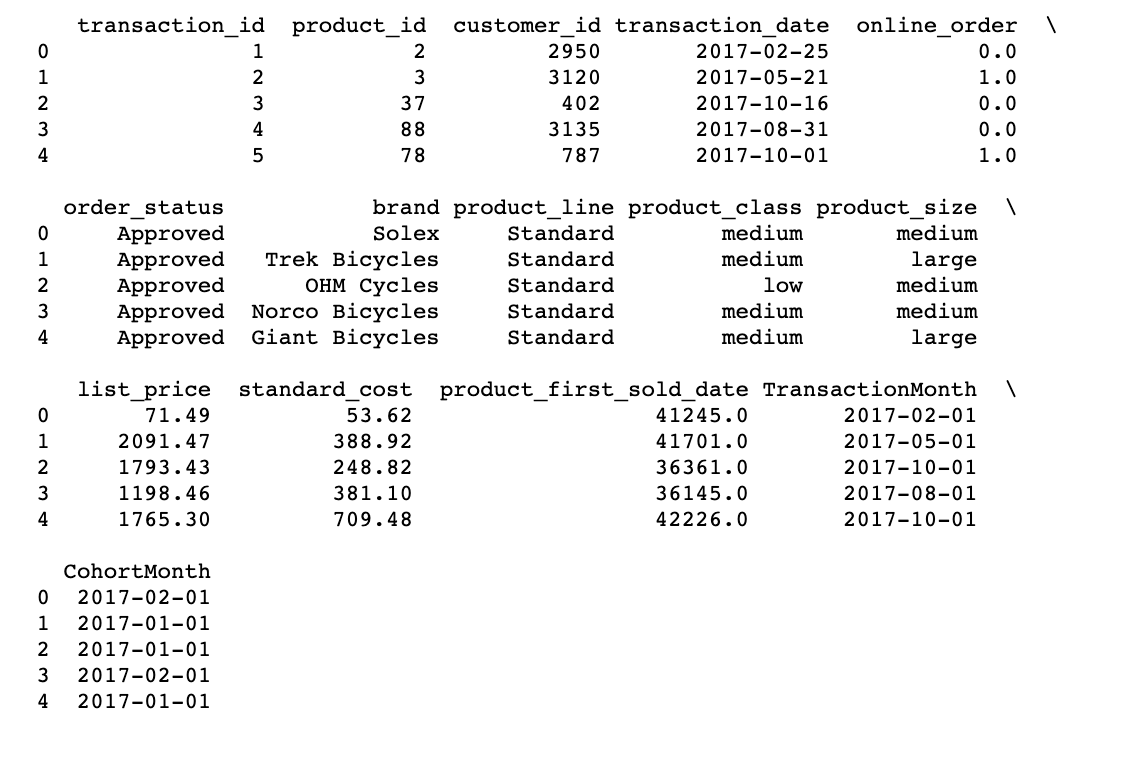
# A function that will parse the date Time based cohort:  1 day of month
def get_month(x): return dt.datetime(x.year, x.month, 1)
# Create transaction_date column based on month and store in TransactionMonth
transaction_df['TransactionMonth'] = transaction_df['transaction_date'].apply(get_month)
# Grouping by customer_id and select the InvoiceMonth value
grouping = transaction_df.groupby('customer_id')['TransactionMonth']
# Assigning a minimum InvoiceMonth value to the dataset
transaction_df['CohortMonth'] = grouping.transform('min')
# printing top 5 rows
print(transaction_df.head())
Cálculo de la compensación de tiempo en el mes como índice de cohorte
Calculating the time compensation for each transaction allows you to evaluate the metrics for each cohort in a comparable way.
First, we will create 6 variables that capture the integer value of years, months and days for Transaction and Cohort Date using the get_date_int function ().
def get_date_int(df, column):
    year = df[column].dt.year
    month = df[column].dt.month
    day = df[column].dt.day
    return year, month, day
# Getting the integers for date parts from the `InvoiceDay` column
transcation_year, transaction_month, _ = get_date_int(transaction_df, 'TransactionMonth')
# Getting the integers for date parts from the `CohortDay` column
cohort_year, cohort_month, _ = get_date_int(transaction_df, 'CohortMonth')
We will now calculate the difference between invoice dates and cohort dates in years, months separately. then calculate the total difference of months between the two. This will be the cohort or compensation index of our month, which we will use in the next section to calculate the retention rate.
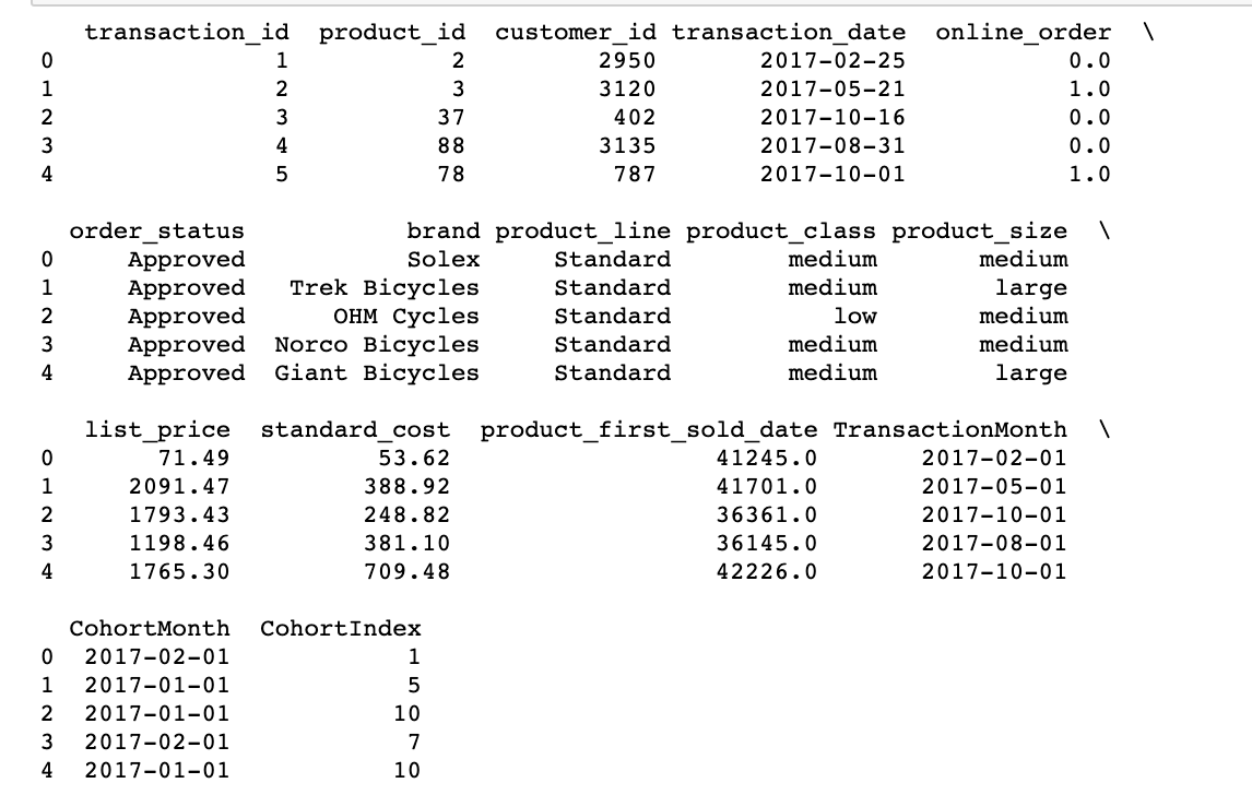
#  Get the  difference in years
years_diff = transcation_year - cohort_year
# Calculate difference in months
months_diff = transaction_month - cohort_month
""" Extract the difference in months from all previous values
 "+1" in addeded at the end so that first month is marked as 1 instead of 0 for easier interpretation.
 """
transaction_df['CohortIndex'] = years_diff * 12 + months_diff  + 1
print(transaction_df.head(5))
Here, at first, we created a group() object with CohortMonth and CohortIndex and save it as a grouping.
Later, we call this object, we select the Customer identification column and calculate the average.
We then store the results as cohort_data. Later, reset the index before calling the pivot function to be able to access the columns now stored as indexes.
Finally, creamos una dynamic tablePivotTable is a powerful tool in spreadsheet programs, such as Microsoft Excel and Google Sheets. Allows you to summarize, Analyze and visualize large volumes of data efficiently. Through its intuitive interface, users can rearrange information, apply filters and create custom reports, facilitating informed decision-making in various contexts, from the business field to academic research.... omitiendo
- CohortMes to the index parameter,
- Cohort index to the column parameter,
- Customer identification to the values parameter.
and round it to 1 digit and see what we get.
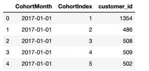
# Counting daily active user from each chort
grouping = transaction_df.groupby(['CohortMonth', 'CohortIndex'])
# Counting number of unique customer Id's falling in each group of CohortMonth and CohortIndex
cohort_data = grouping['customer_id'].apply(Pd. Series.nunique)
cohort_data = cohort_data.reset_index()
 # Assigning column names to the dataframe created above
cohort_counts = cohort_data.pivot(index='CohortMonth',
                                 columns="CohortIndex",
                                 values="customer_id")
# Printing top 5 rows of Dataframe
cohort_data.head()
Calculate business metrics: retention rate
The percentage of active customers compared to the total number of customers after a specified time interval is called the retention rate..
In this section, we will calculate the retention count for each cohort month matched with the cohort index
Now that we have a count of the retained customers for each cohorteMes Y cohortIndex. We will calculate the retention rate for each cohort.
We will create a pivot table for this purpose.
cohort_sizes = cohort_counts.iloc[:,0]
retention = cohort_counts.divide(cohort_sizes, axis=0)
# Coverting the retention rate into percentage and Rounding off.
retention.round(3)*100
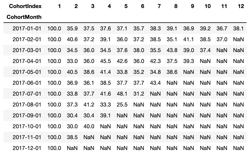
Retention Rate Data Frame Represents Retained Customer Across All Cohorts. We can read it as follows:
- The index value represents the cohort
- The columns represent the number of months since the current cohort
For instance: The value in CohortMonth 2017-01-01, CohortIndex 3 it is 35,9 and represents 35,9% of clients in the cohort 2017-01 were held in the 3is mes.
What's more, you can see in the DataFrame for retention rate:
- Retention rate The first index, namely, the first month is from 100%, since all clients of that particular client signed up in the first month
- The retention rate can increase or decrease in subsequent indices.
- Values towards the lower right have many NaN values.
Visualizing the retention rate
Before we start to draw our heat map, let's set the index of our retention rate data frame to a more readable string format.
average_standard_cost.index = average_standard_cost.index.strftime('%Y-%m')
# Initialize the figure
plt.figure(figsize=(16, 10))
# Adding a title
plt.title('Average Standard Cost: Monthly Cohorts', fontsize = 14)
# Creating the heatmap
sns.heatmap(average_standard_cost, annot = True,vmin = 0.0, vmax =20,cmap="YlGnBu", fmt="g")
plt.ylabel('Cohort Month')
plt.xlabel('Cohort Index')
plt.yticks( rotation='360')
plt.show()
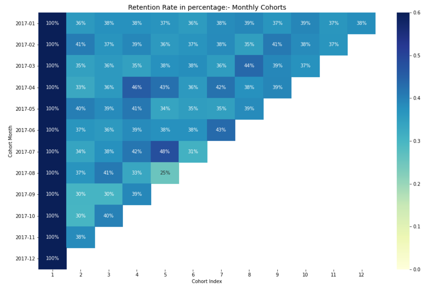
Interpreting the retention rate
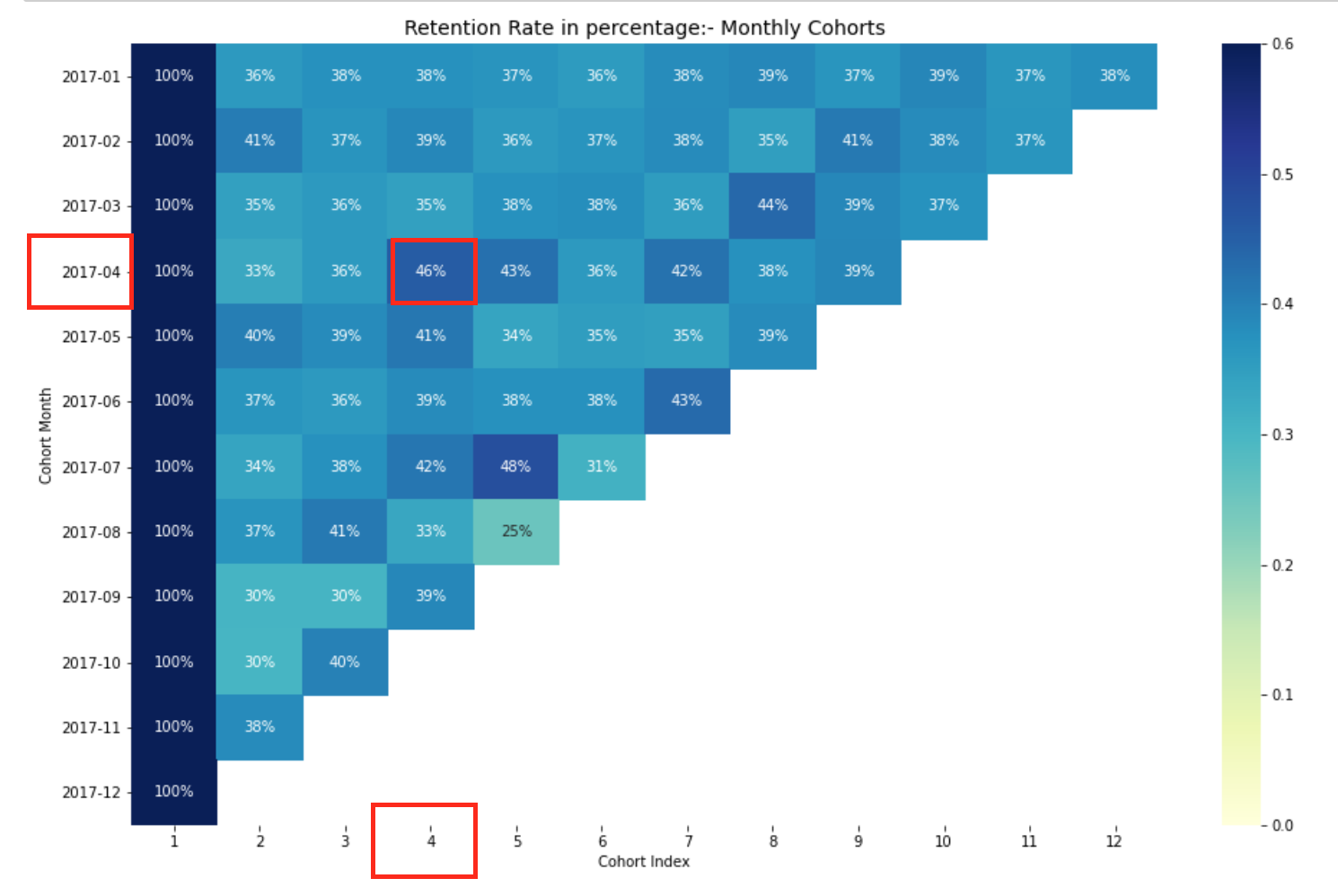
The most effective way to visualize and analyze cohort analysis data is through a heat map., as we did previously. Provides both actual metric values and color coding to see differences in numbers visually.
If you don't have a basic knowledge about heatmap, you can check my blog. Exploratory data analysis for beginners with Python, where I have talked about heat maps for beginners.
Here, have 12 cohorts for each month and 12 cohort indices. The darker the shades of blue, the higher the values. A) Yes, if we see in the month of the cohort 2017-07 in the 5th cohort index, we see the dark blue tone with a 48% which means that the 48% of the cohorts that signed in July 2017 they were active 5 months later.
This concludes our cohort analysis for the retention rate.. Similarly, we can perform cohort analysis for other commercial matrices.
Click here to learn more about cohort analysis for companies free with DataCamp.(Affiliate link)
Therefore, we completed our Cohort Analysis, where you learned about basic and cohort analyzes, conducting time cohorts, working with pandas pivot and creating a hold table along with visualization. We also learned how to explore other matrices.
Now, you can start creating and exploring the metrics that are important to your business on your own.
The media shown in this article is not the property of DataPeaker and is used at the author's discretion.


