Introduction
When it starts with data science, starts out simple. You go through simple projects like Loan prediction problem O Big Mart Sales Prediction. These problems have structured data arranged neatly in a tabular format. In other words, You are spoon fed the hardest part in the data science pipeline.

Data sets in real life are much more complex.
You must understand it first, collect it from various sources and organize it in a format that is ready for processing. This is even more difficult when the data is in an unstructured format, as an image or an audio. This is so because it would have to represent image data / audio in a standard way to be useful for analysis.
The abundance of unstructured data
curiously, unstructured data represents a great little-exploited opportunity. It's closer to how we communicate and interact as humans. It also contains a lot of useful and powerful information. For instance, if a person speaks; you don't just get what it says, but also what were the emotions of the person from the voice.
What's more, the person's body language can show you many more characteristics about a person, Because actions speak louder than words! In summary, unstructured data is complex, but processing them can yield easy rewards.
In this article, I intend to cover an overview of audio processing / voz con un estudio de caso para que pueda obtener una introducción práctica a la resolutionThe "resolution" refers to the ability to make firm decisions and meet set goals. In personal and professional contexts, It involves defining clear goals and developing an action plan to achieve them. Resolution is critical to personal growth and success in various areas of life, as it allows you to overcome obstacles and keep your focus on what really matters.... de problemas de procesamiento de audio.
Let's move on!
Table of Contents
- What do you mean by audio data?
- Audio processing applications
- Data handling in the audio domain
- Let's solve the UrbanSound challenge!!
- Intermediate: our first presentation
- Let's solve the challenge! Part 2: Building better models
- Future steps to explore
What do you mean by audio data?
Directly or indirectly, you are always in touch with the audio. Your brain continuously processes and understands audio data and provides you with information about the environment. A simple example can be your conversations with people that you do on a daily basis.. This speech is discerned by the other person to continue the discussions. Even when you think you are in a quiet environment, tends to pick up much more subtle sounds, like the rustle of leaves or the splash of rain. This is the extent of your connection to audio.
Then, Can you somehow capture this audio floating around you to do something constructive? Yes, of course! There are built-in devices that help you pick up these sounds and represent them in a computer-readable format.. Examples of these formats are
- wav format (waveform audio file)
- formato mp3 (MPEG-1 Audio Layer 3)
- WMA format (Windows Media Audio)
If you think about what an audio looks like, it is nothing more than a waveform data format, where the amplitude of the audio changes with respect to time. This can be pictorially represented as follows.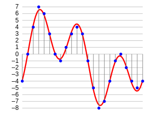
Audio processing applications
Although we comment that the audio data can be useful for the analysis. But, What are the possible applications of audio processing? Here I would list some of them.
- Indexing of music collections based on their audio characteristics.
- Recommend music for radio channels
- Finding Similarities for Audio Files (aka Shazam)
- Speech processing and synthesis: artificial voice generation for conversational agents
Here is an exercise; Can you think of an audio processing app that can potentially help thousands of lives?
Data handling in the audio domain
As with all unstructured data formats, audio data has a couple of preprocessing steps that must be followed before it is presented for analysis. We will cover this in detail in a later article., here we will get an insight as to why this is done.
The first step is to load the data in a machine understandable format. For this, we just take values after each specific time step. For instance; in an audio file of 2 seconds, we extract values at half a second. Is named audio data sampling, and the rate at which it is sampled is called sampling rate.
Another way to represent audio data is to convert it to a different data representation domain, namely, the frequency domain. When we sample audio data, we need many more data points to represent all the data and, what's more, the sampling frequency should be as high as possible.
Secondly, if we represent audio data in frequency domain, much less computational space is required. To have an intuition, take a look at the picture below.
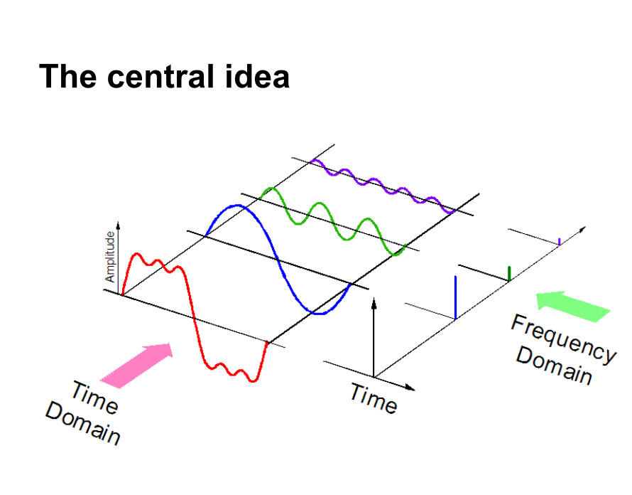
Here, we separate an audio signal into 3 different pure signals, which can now be represented as three unique values in the frequency domain.
There are a few more ways that audio data can be represented, for instance. using MFC (honey frequency cepstrums. PD: We will cover this in the later article.). These are just different ways of representing the data.
Now, the next step is to extract features from these audio representations, so that our algorithm can work on these characteristics and perform the task for which it is designed. Then, a visual representation of the categories of audio functions that can be extracted is shown.
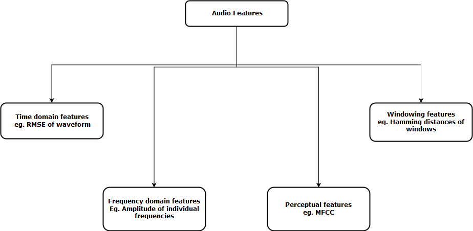
After extracting these features, sent to the machine learning model for further analysis.
Let's solve the UrbanSound challenge!!
Let's get a better practical overview on a real life project, the Urban sound challenge. This practice problem is intended to introduce you to audio processing in the typical classification scenario.
The data set contains 8732 sound excerpts (<= 4 s) of urban sounds of 10 lessons, namely:
- air conditioning,
- Horn,
- children playing,
- dog barking,
- drilling,
- Engine idle,
- gun shot
- pneumatic hammer,
- mermaid and
- Street Music
Here's a extractThe extract is a substance obtained by concentrating compounds of plant origin, animal or mineral. Used in a variety of applications, such as the food industry, Pharmaceutical & Cosmetics. Extracts can be presented in liquid form, in powder form or as tinctures, and its production involves techniques such as maceration, distillation or solvent extraction. Its use allows to take advantage of the beneficial properties of the original ingredients in a more way.. de sonido del conjunto de datos. Can you guess what class it belongs to?
To reproduce this in jupyter's notebook, you can just follow the code.
import IPython.display as ipd
ipd.Audio('../data/Train/2022.wav')
Now let's load this audio into our laptop as a large matrix. For this we will use books python library. To install books, just type this in the command line
pip install librosaNow we can run the following code to load the data.
data, sampling_rate = librosa.load('../data/Train/2022.wav')
When you load the data, gives you two objects; a large array of an audio file and the corresponding sample rate by which it was extracted. Now, to represent this as a waveform (which is originally), use the following code
% pylab inline
import os
import pandas as pd
import librosa
import glob

plt.figure(figsize=(12, 4))
librosa.display.waveplot(data, sr=sampling_rate)
The output goes as follows
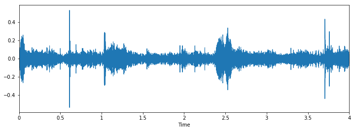
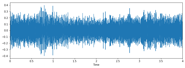
Now let's visually inspect our data and see if we can find patterns in the data..
Class: jackhammerClass: drilling
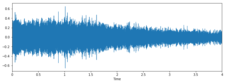
 Class: drilling
 Class: dog_barking
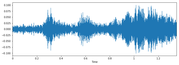
We can see that it can be difficult to differentiate between pneumatic hammer and drilling, but it's still easy to distinguish between dog barking and piercing. To see more examples of this type, you can use this code
i = random.choice(train.index)

audio_name = train.ID[i]
path = os.path.join(data_dir, 'Train', str(audio_name) + '.wav')

print('Class: ', train.Class[i])
x, sr = librosa.load('../data/Train/' + str(train.ID[i]) + '.wav')

plt.figure(figsize=(12, 4))
librosa.display.waveplot(x, sr=sr)
Intermediate: our first presentation
We will do a similar approach as we did for the age detection problem, to see the class distributions and only predict the maximum occurrence of all test cases as that class.
Let's look at the distributions for this problem.
train.Class.value_counts()
Out[10]:

jackhammer 0.122907
engine_idling 0.114811
siren 0.111684
dog_bark 0.110396
air_conditioner 0.110396
children_playing 0.110396
street_music 0.110396
drilling 0.110396
car_horn 0.056302
gun_shot 0.042318
We see that the pneumatic hammer class has more values than any other class. So let's create our first presentation with this idea.
test = pd.read_csv('../data/test.csv')
test['Class'] = 'jackhammer'
test.to_csv(‘sub01.csv’, index=False)
This seems like a good idea as a benchmark for any challenge, but for this problem, seems a bit unfair. This is because the data set is not very unbalanced.
Let's solve the challenge! Part 2: Building better models
Now let's see how we can take advantage of the concepts we learned earlier to solve the problem.. We will follow these steps to fix the problem.
Paso 1: upload audio files
Paso 2: extract functions from audio
Paso 3: convierta los datos para pasarlos en nuestro modelo de deep learningDeep learning, A subdiscipline of artificial intelligence, relies on artificial neural networks to analyze and process large volumes of data. This technique allows machines to learn patterns and perform complex tasks, such as speech recognition and computer vision. Its ability to continuously improve as more data is provided to it makes it a key tool in various industries, from health...
Paso 4: Run a deep learning model and get results
Below is a code of how I implemented these steps
Paso 1 Y 2 combined: load audio files and extract functions
def parser(row):
   # function to load files and extract features
   file_name = os.path.join(os.path.abspath(data_dir), 'Train', str(row.ID) + '.wav')

   # handle exception to check if there isn't a file which is corrupted
   try:
      # here kaiser_fast is a technique used for faster extraction
      X, sample_rate = librosa.load(file_name, res_type="kaiser_fast")
      # we extract mfcc feature from data
      mfccs = np.mean(librosa.feature.mfcc(y = X, sr=sample_rate, n_mfcc=40).T,axis=0)
   except Exception as e:
      print("Error encountered while parsing file: ", file)
      return None, None

   feature = mfccs
   label = row.Class

   return [feature, label]

temp = train.apply(parser, axis=1)
temp.columns = ['feature', 'label']
Paso 3: convert data to pass into our deep learning model
from sklearn.preprocessing import LabelEncoder

X = np.array(temp.feature.tolist())
y = np.array(temp.label.tolist())

lb = LabelEncoder()

y = np_utils.to_categorical(lb.fit_transform(Y))
Paso 4: Run a deep learning model and get results
import numpy as np
from keras.models import Sequential
from keras.layers import Dense, Dropout, Activation, Flatten
from keras.layers import Convolution2D, MaxPooling2D
from keras.optimizers import Adam
from keras.utils import np_utils
from sklearn import metrics

num_labels = y.shape[1]
filter_size = 2

# build model
model = Sequential()

model.add(Dense(256, input_shape=(40,)))
model.add(Activation('relu'))
model.add(Dropout(0.5))

model.add(Dense(256))
model.add(Activation('relu'))
model.add(Dropout(0.5))

model.add(Dense(num_labels))
model.add(Activation('softmax'))

model.compile(loss="categorical_crossentropy", metrics=['accuracy'], optimizer="adam")
Now let's train our model
model.fit(X, Y, batch_size=32, epochs=5, validation_data=(val_x, val_y))
This is the result I got from training during 5 epochs
Train on 5435 samples, validate on 1359 samples
Epoch 1/10
5435/5435 [==============================] - 2s - loss: 12.0145 - acc: 0.1799 - val_loss: 8.3553 - val_acc: 0.2958
Epoch 2/10
5435/5435 [==============================] - 0s - loss: 7.6847 - acc: 0.2925 - val_loss: 2.1265 - val_acc: 0.5026
Epoch 3/10
5435/5435 [==============================] - 0s - loss: 2.5338 - acc: 0.3553 - val_loss: 1.7296 - val_acc: 0.5033
Epoch 4/10
5435/5435 [==============================] - 0s - loss: 1.8101 - acc: 0.4039 - val_loss: 1.4127 - val_acc: 0.6144
Epoch 5/10
5435/5435 [==============================] - 0s - loss: 1.5522 - acc: 0.4822 - val_loss: 1.2489 - val_acc: 0.6637
Seems to be fine, but obviously you can increase the score. (PD: could get precision from 80% in my validation dataset). Now is your turn, Can you increase this score? If so, Let me know in the comments below!!
Future steps to explore
Now that we saw simple applications, we can come up with some more methods that can help us improve our score.
- Aplicamos un modelo de red neuronalNeural networks are computational models inspired by the functioning of the human brain. They use structures known as artificial neurons to process and learn from data. These networks are fundamental in the field of artificial intelligence, enabling significant advancements in tasks such as image recognition, Natural Language Processing and Time Series Prediction, among others. Their ability to learn complex patterns makes them powerful tools.. simple al problema. Our next immediate step should be understand where the model fails and why. With this, we want to conceptualize our understanding of algorithm flaws so that the next time we build a model, don't make the same mistakes.
- We can build more efficient models that our “best models”, such as convolutional neural networks or recurrent neural networks. These models have been shown to solve these types of problems more easily.
- We touched on the concept of data augmentation, but we don't apply them here. You can try it to see if it works for the problem.
Final notes
In this article, I have provided a short overview of audio processing with a case study on the UrbanSound challenge. I have also shown the steps you do when dealing with audio data in python with the package books. With this “shastra” in your hand, hope you can test your own algorithms in Urban Sound challenge, or try to solve your own audio problems in daily life. If you have any suggestions / idea, let me know in the comments below.
Learn, engage , chop and get hired!

Podcast: Play in new window | Descargar