
Introduction
Have you ever come across a dataset or an image and wondered if you could create a system capable of differentiating or identifying the image??
The concept of image classification will help us with that.. Image classification is one of the most popular applications of computer vision and a must-have concept for anyone looking to play a role in this field..
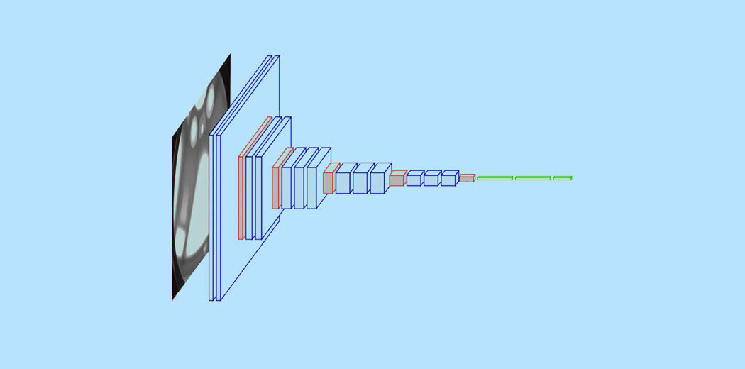
In this article, We will see a very simple but widely used application that is Image Classification. We will not only see how to make a simple and efficient model to classify the data, but we will also learn how to implement a previously trained model and compare the performance of the two.
At the end of the article, you will be able to find your own dataset and implement image classification with ease.
Prerequisites before starting:
Sounds interesting? So get ready to create your own image classifier!!
Table of Contents
- Image classification
- Understanding the problem statement
- Image data settings
- Let's build our image classification model
- Data preprocessing
- Data augmentation
- Definition and formation of the model
- Evaluation of results
- The art of transferred learning
- Import MobileNetV2 Base Model
- Sintonia FINA
- Training
- Evaluation of results
- Whats Next?
What is image classification?
Image classification is the task of assigning an input image, a tag from a fixed set of categories. This is one of the central problems of Computer Vision that, despite its simplicity, has a wide variety of practical applications.
Let's take an example to understand it better. When we do the image classification, our system will receive an image as input, for instance, a cat. Now the system will know a set of categories and its objective is to assign a category to the image.
This problem may seem simple or easy, but it is very difficult problem for computer to solve. How will you know, the computer sees a grid of numbers and not the image of a cat as we see it. The images are three-dimensional arrays of integers of 0 a 255, in size Width x Height x 3. The 3 represents the three channels in Red, Verde, Blue.
Then, How can our system learn to identify this image? By using convolutional neural networks. Las redes neuronales convolucionales o CNN son una clase de redes neuronales de deep learningDeep learning, A subdiscipline of artificial intelligence, relies on artificial neural networks to analyze and process large volumes of data. This technique allows machines to learn patterns and perform complex tasks, such as speech recognition and computer vision. Its ability to continuously improve as more data is provided to it makes it a key tool in various industries, from health... que representan un gran avance en el reconocimiento de imágenes. You may already have a basic understanding of CNN, and we know that CNN consist of convolutional layers, covers resumeThe ReLU activation function (Rectified Linear Unit) It is widely used in neural networks due to its simplicity and effectiveness. Defined as ( f(x) = max(0, x) ), ReLU allows neurons to fire only when the input is positive, which helps mitigate the problem of gradient fading. Its use has been shown to improve performance in various deep learning tasks, making ReLU an option..., clustered layers and fully connected dense layers.
To read about Image Classification and CNN in detail, you can consult the following resources: –
- https://www.analyticsvidhya.com/blog/2020/02/learn-image-classification-cnn-convolutional-neural-networks-3-datasets/
- https://www.analyticsvidhya.com/blog/2019/01/build-image-classification-model-10-minutes/
Now that we understand the concepts, let's dive into how an image classification model can be built and how it can be implemented.
Understanding the problem statement
Consider the following image:
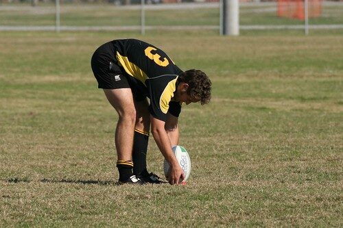
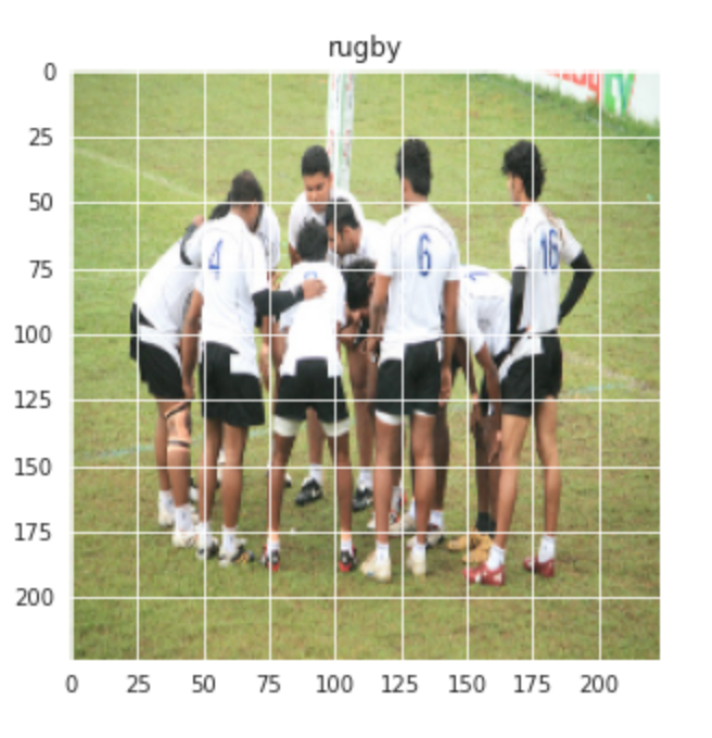
A person well versed in sports will be able to recognize the image as Rugby. There may be different aspects of the image that helped you identify it as Rugby, it could be the shape of the ball or the player's outfit. But did you notice that this image could very well be identified as a soccer image?
Let's consider another image: –
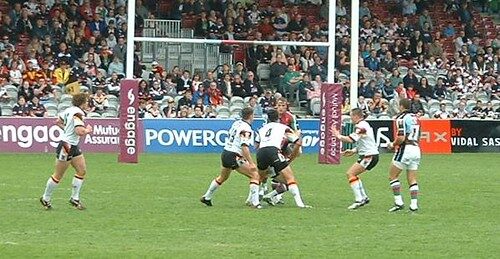
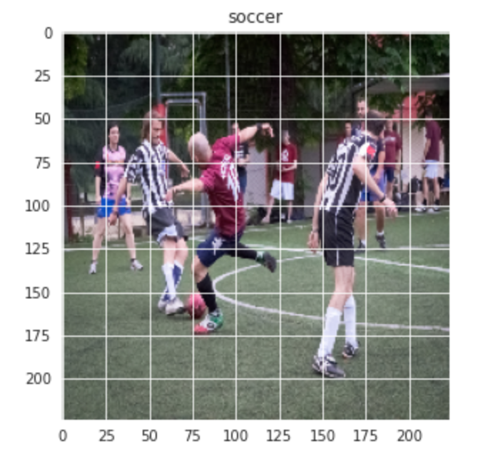
What do you think this image represents? Hard to guess, truth? The image to the inexperienced human eye can easily be misclassified as football, But actually, it's a rugby image, since we can see that the goal post behind is not a net and is larger. The question now is whether we can make a system that can possibly classify the image correctly.
That is the idea behind our project here, we want to build a system that is capable of identifying the sport represented in that image. The two classification classes here are Rugby and Soccer. Posing the problem can be a bit tricky as sports have many aspects in common, but nevertheless, we will learn how to tackle the problem and create a good performing system.
Configuration of our image data
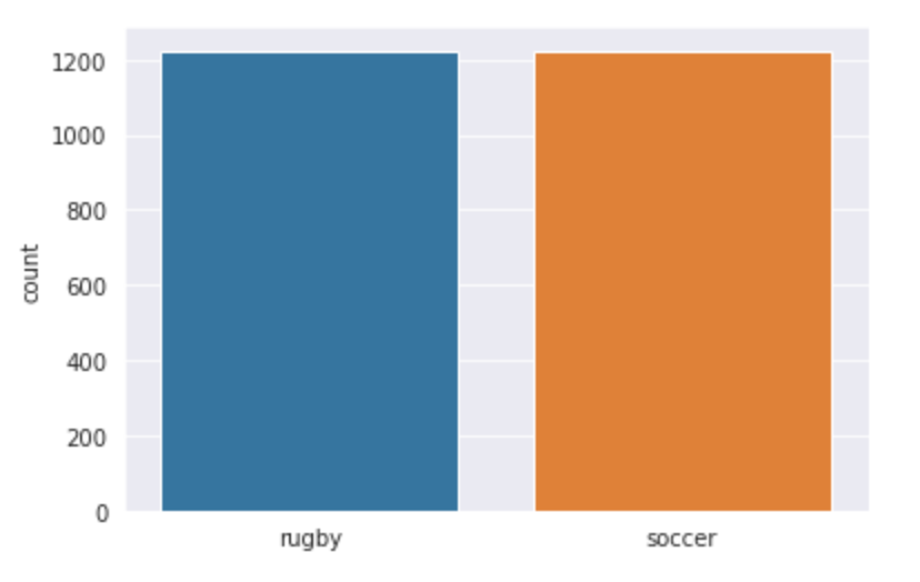
Since we are working on an image classification problem, I have used two of the largest sources of image data, namely, ImageNet y Google OpenImages. I implemented two python scripts so that we can download the images easily. A total of 3058 images, that were divided into train and test. I did a split 80-20 with the train folder I had 2448 images and the test folder has 610. Both Rugby and Soccer classes have 1224 images each.
Our data structure is as follows: –
- Entry – 3058
- Train – 2048
- Rugby – 1224
- Soccer – 1224
- Train – 2048
-
- Test – 610
- Rugby – 310
- Soccer – 310
- Test – 610
Let's build our image classification model!
Paso 1: – Import the required libraries
Here we will use the Keras library to create our model and train it. We also use Matplotlib and Seaborn to visualize our dataset and get a better understanding of the images we are going to handle.. Another important library for handling image data is Opencv.
import matplotlib.pyplot as plt
import seaborn as sns

import keras
from keras.models import Sequential
from keras.layers import Dense, Conv2D , MaxPool2D , Flatten , Dropout
from keras.preprocessing.image import ImageDataGenerator
from keras.optimizers import Adam

from sklearn.metrics import classification_report,confusion_matrix

import tensorflow as tf

import cv2
import os

import numpy as np
Paso 2: – Loading the data
Then, let's define the path to our data. Let's define a function called get_data () to make it easier for us to create our train and validation data set. We define the two labels ‘Rugby’ and soccer’ what will we use. We use Opencv's imread function to read the images in RGB format and resize the images to our desired width and height, in this case both are 224.
labels = ['rugby', 'soccer']
img_size = 224
def get_data(data_dir):
    data = []
    for label in labels:
        path = os.path.join(data_dir, label)
        class_num = labels.index(label)
        for img in os.listdir(path):
            try:
                img_arr = cv2.imread(os.path.join(path, img))[...,::-1] #convert BGR to RGB format
                resized_arr = cv2.resize(img_arr, (img_size, img_size)) # Reshaping images to preferred size
                data.append([resized_arr, class_num])
            except Exception as e:
                print(e)
    return np.array(data)
Now we can easily fetch our train and validation data.
train = get_data('.. /input/traintestsports/Main/train')
val = get_data('.. /input/traintestsports/Main/test')
Paso 3: – Visualize the data
Let's visualize our data and see what exactly we are working with. We use seaborn to plot the number of images in both classes and you can see what the output looks like.
l = []
for i in train:
    if(i[1] == 0):
        l.append("rugby")
    else
        l.append("soccer")
sns.set_style('darkgrid')
sns.countplot(l)
Production:
Let's also visualize a random image of the Rugby and Soccer classes: –
plt.figure(figsize = (5,5))
plt.imshow(train[1][0])
plt.title(labels[train[0][1]])
Production:-
Similarly for the soccer image: –
plt.figure(figsize = (5,5))
plt.imshow(train[-1][0])
plt.title(labels[train[-1][1]])
Production:-
Paso 4: – Data preprocessing and augmentation
Then, we do a bit of preprocessing and data augmentation before we can proceed with building the model.
x_train = []
y_train = []
x_val = []
y_val = []

for feature, label in train:
  x_train.append(feature)
  y_train.append(label)

for feature, label in val:
  x_val.append(feature)
  y_val.append(label)

# Normalize the data
x_train = np.array(x_train) / 255
x_val = np.array(x_val) / 255

x_train.reshape(-1, img_size, img_size, 1)
y_train = np.array(y_train)

x_val.reshape(-1, img_size, img_size, 1)
y_val = np.array(y_val)
Increase in data on train data: –
datagen = ImageDataGenerator(
        featurewise_center=False,  # set input mean to 0 over the dataset
        samplewise_center=False,  # set each sample mean to 0
        featurewise_std_normalization=False,  # divide inputs by std of the dataset
        samplewise_std_normalization=False,  # divide each input by its std
        zca_whitening=False,  # apply ZCA whitening
        rotation_range = 30,  # randomly rotate images in the range (degrees, 0 to 180)
        zoom_range = 0.2, # Randomly zoom image
        width_shift_range=0.1,  # randomly shift images horizontally (fraction of total width)
        height_shift_range=0.1,  # randomly shift images vertically (fraction of total height)
        horizontal_flip = True,  # randomly flip images
        vertical_flip=False)  # randomly flip images


datagen.fit(x_train)
Paso 5: – Define the model
Let's define a simple CNN model with 3 convolutional layers followed by layers of maximum grouping. A drop layer is added after the third maxpool operation to prevent overfitting.
model = Sequential()
model.add(Conv2D(32,3,padding="same", activation="resume", input_shape=(224,224,3)))
model.add(MaxPool2D())

model.add(Conv2D(32, 3, padding="same", activation="resume"))
model.add(MaxPool2D())

model.add(Conv2D(64, 3, padding="same", activation="resume"))
model.add(MaxPool2D())
model.add(Dropout(0.4))

model.add(Flatten())
model.add(Dense(128,activation="resume"))
model.add(Dense(2, activation="softmax"))

model.summary()
Let's compile the model now using Adam as our optimizer and SparseCategoricalCrossentropy as the Loss functionThe loss function is a fundamental tool in machine learning that quantifies the discrepancy between model predictions and actual values. Its goal is to guide the training process by minimizing this difference, thus allowing the model to learn more effectively. There are different types of loss functions, such as mean square error and cross-entropy, each one suitable for different tasks and.... We are using a lower learning rate of 0.000001 for a smoother curve.
opt = Adam(lr=0.000001)
model.compile(optimizer = opt , loss = tf.keras.losses.SparseCategoricalCrossentropy(from_logits=True) , metrics = ['accuracy'])
Now, let's train our model during 500 epochs, since our learning rate is very small.
history = model.fit(x_train,y_train,epochs = 500 , validation_data = (x_val, y_val))
Paso 6: – Evaluation of the result
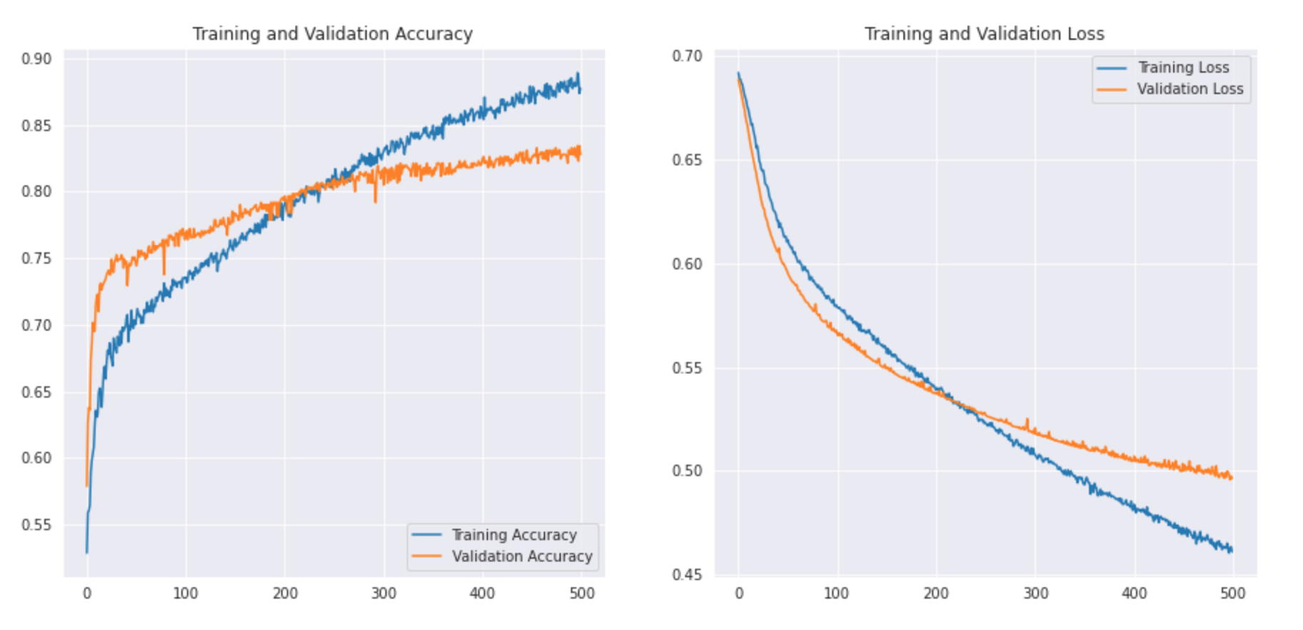
We'll map out our accuracy of trainingTraining is a systematic process designed to improve skills, physical knowledge or abilities. It is applied in various areas, like sport, Education and professional development. An effective training program includes goal planning, regular practice and evaluation of progress. Adaptation to individual needs and motivation are key factors in achieving successful and sustainable results in any discipline.... and validation along with loss of training and validation.
acc = history.history['accuracy']
val_acc = history.history['val_accuracy']
loss = history.history['loss']
val_loss = history.history['val_loss']

epochs_range = range(500)

plt.figure(figsize=(15, 15))
plt.subplot(2, 2, 1)
plt.plot(epochs_range, acc, label="Training Accuracy")
plt.plot(epochs_range, val_acc, label="Validation Accuracy")
plt.legend(loc ="lower right")
plt.title('Training and Validation Accuracy')

plt.subplot(2, 2, 2)
plt.plot(epochs_range, loss, label="Training Loss")
plt.plot(epochs_range, val_loss, label="Validation Loss")
plt.legend(loc ="upper right")
plt.title('Training and Validation Loss')
plt.show()
Let's see what the curve looks like: –
We can print the classification report to see the precision and accuracy.
predictions = model.predict_classes(x_val)
predictions = predictions.reshape(1,-1)[0]
print(classification_report(y_val, predictions, target_names = ['Rugby (Class 0)','Soccer (Class 1)']))
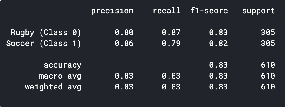
As we can see, our simple CNN model was able to achieve an accuracy of the 83%. With some hyperparameter settings, we could achieve a precision of 2-3%.
We can also visualize some of the incorrectly predicted images and see where our classifier is failing.
The art of transferred learning
Let's first see what transfer learning is. Transfer learning is a machine learning technique in which a model trained on one task is redirected to a second related task. Another crucial application of transfer learning is when the data set is small, By using a previously trained model on similar images we can easily achieve high performance. Since our problem statement is a good fit for transfer learning, let's see how we can implement a pre-trained model and what precision we can achieve.
Paso 1: – Import the model
We will create a base model from the MobileNetV2 model. This is pre-trained on the ImageNet dataset, a large data set consisting of 1,4 million images and 1000 lessons. This knowledge base will help us classify rugby and football from our specific data set..
By specifying the include_top = False argument, loads a network that does not include the classification layers on top.
base_model = tf.keras.applications.MobileNetV2(input_shape = (224, 224, 3), include_top = False, weights = "imagenet")
It is important to freeze our database before compiling and training the model. Freezing will prevent our base model weights from updating during training.
base_model.trainable = False
Then, we define our model using our base_model followed by a GlobalAveragePooling function to convert the features to a single vector per image. We add a dropout of 0.2 and the dense layerThe dense layer is a geological formation that is characterized by its high compactness and resistance. It is commonly found underground, where it acts as a barrier to the flow of water and other fluids. Its composition varies, but it usually includes heavy minerals, which gives it unique properties. This layer is crucial in geological engineering and water resources studies, since it influences the availability and quality of water.. final with 2 neurons and softmax activation.
model = tf.keras.Sequential([base_model,
                                 tf.keras.layers.GlobalAveragePooling2D(),
                                 tf.keras.layers.Dropout(0.2),
                                 tf.hard.layers.Dense(2, activation="softmax")
                                ])
Then, let's compile the model and start training it.
base_learning_rate = 0.00001
model.compile(optimizer=tf.hard.optimizers.Adam(lr=base_learning_rate),
              loss=tf.keras.losses.BinaryCrossentropy(from_logits=True),
              metrics=['accuracy'])

history = model.fit(x_train,y_train,epochs = 500 , validation_data = (x_val, y_val))
Paso 2: – Evaluation of the result.
acc = history.history['accuracy']
val_acc = history.history['val_accuracy']
loss = history.history['loss']
val_loss = history.history['val_loss']
epochs_range = range(500)

plt.figure(figsize=(15, 15))
plt.subplot(2, 2, 1)
plt.plot(epochs_range, acc, label="Training Accuracy")
plt.plot(epochs_range, val_acc, label="Validation Accuracy")
plt.legend(loc ="lower right")
plt.title('Training and Validation Accuracy')

plt.subplot(2, 2, 2)
plt.plot(epochs_range, loss, label="Training Loss")
plt.plot(epochs_range, val_loss, label="Validation Loss")
plt.legend(loc ="upper right")
plt.title('Training and Validation Loss')
plt.show()
Let's see what the curve looks like: –
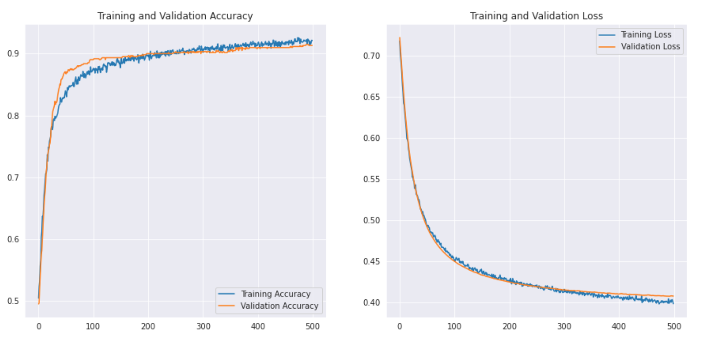
We also print the classification report to obtain more detailed results.
predictions = model.predict_classes(x_val)
predictions = predictions.reshape(1,-1)[0]

print(classification_report(y_val, predictions, target_names = ['Rugby (Class 0)','Soccer (Class 1)']))
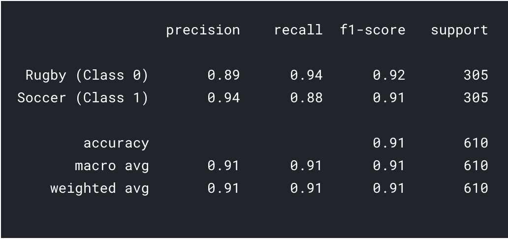
As we can see with transfer learning, we were able to get a much better result. Both Rugby and Soccer accuracy are higher than our CNN model and also the overall accuracy reached the 91%, what is really good for such a small data set. With a little hyperparameter tuning and changes of parametersThe "parameters" are variables or criteria that are used to define, measure or evaluate a phenomenon or system. In various fields such as statistics, Computer Science and Scientific Research, Parameters are critical to establishing norms and standards that guide data analysis and interpretation. Their proper selection and handling are crucial to obtain accurate and relevant results in any study or project...., We could also achieve a little better performance!!
Whats Next?
This is just the starting point in the field of computer vision.. In fact, try to improve your basic CNN models to meet or exceed benchmark performance.
- You can learn from VGG16 architectures, etc. for some hints on hyperparameter tuning.
- You can use the same ImageDataGenerator to increase your images and increase the size of the dataset.
- What's more, you can try to implement newer and better architectures like DenseNet and XceptionNet.
- You can also move on to other computer vision tasks, such as detection and segmentationSegmentation is a key marketing technique that involves dividing a broad market into smaller, more homogeneous groups. This practice allows companies to adapt their strategies and messages to the specific characteristics of each segment, thus improving the effectiveness of your campaigns. Targeting can be based on demographic criteria, psychographic, geographic or behavioral, facilitating more relevant and personalized communication with the target audience.... of objects, which you will later realize that it can also be reduced to image classification.
Final notes
Congratulations, you have learned how to create your own dataset and create a CNN model or do transfer learning to solve a problem. We learned a lot in this article, from learning how to search image data to creating a simple CNN model that was able to achieve reasonable performance. We also learned the application of transfer learning to further improve our performance.
That's not the end, we saw that our models misclassified many images, which means that there are still marginMargin is a term used in a variety of contexts, such as accounting, Economics and printing. In accounting, refers to the difference between revenue and costs, which allows the profitability of a business to be evaluated. In the publishing field, The margin is the white space around the text on a page, that makes it easy to read and provides an aesthetic presentation. Its correct management is essential.. of improvement. We could start by finding more data or even implementing newer and better architectures that might be better at identifying features.
Do you find helpful this article? Do share your valuable feedback in the comment section below.. Feel free to share your complete codebooks as well, that will be useful to members of our community.





