This article was published as part of the Data Science Blogathon.
Introduction
A popular and widely used statistical method for time series forecasting is the ARIMA model.. Exponential smoothing and ARIMA models are the two most widely used approaches to time series prediction and provide complementary approaches to the problem.. While exponential smoothing models are based on a description of the trend and seasonality of the data, ARIMA models aim to describe autocorrelations in the data.
To know the seasonality, check this blog.
Before talking about the ARIMA model, Let's talk about the concept of stationarity and the technique of differentiating time series.
Stationarity
A stationary time series data is one whose properties do not depend on time, hence the time series with trends, or with seasonality, they are not stationary. trend and seasonality will affect the time series value at different times. Secondly, for stationarity it doesn't matter when you look at it, should look very similar at any time. In general, a stationary time series will not have predictable long-term patterns.
ARIMA is an acronym for Auto-Regressive Integrated Moving Average. It is a model class that captures a set of different standard temporal structures in time series data.
In this tutorial, we will talk about how to develop an ARIMA model for time series forecasting in Python.
An ARIMA model is a class of statistical models for analyzing and forecasting time series data. It is really simplified in terms of its use. But nevertheless, this model is really powerful.
ARIMA stands for Auto-Regressive Integrated Moving Average.
The ARIMA model parameters are defined as follows:
p: The number of lag observations included in the model, also called lag order.
d: The number of times raw observations differ, also called degree of difference.
q: The size of the moving average window, also called moving average order.
A linear regression model is constructed that includes the specified number and type of terms, and the data is prepared by a degree of differentiation to make it stationary, namely, eliminate trend and seasonal structures that adversely affect the regression model.
STEPS
1. View time series data
2. Identify if the date is stationary
3. Plot the correlation and automatic correlation graphs
4. Build the ARIMA or seasonal ARIMA model based on the data
Let us begin
import numpy as np
import pandas as pd
import matplotlib.pyplot as plt
%matplotlib inline
In this tutorial, I'm using the following dataset.
df=pd.read_csv('time_series_data.csv')
df.head()

# Updating the header
df.columns=["Month","Sales"]
df.head()
df.describe()
df.set_index('Month',inplace=True)

from pylab import rcParams
rcParams['figure.figsize'] = 15, 7
df.plot()
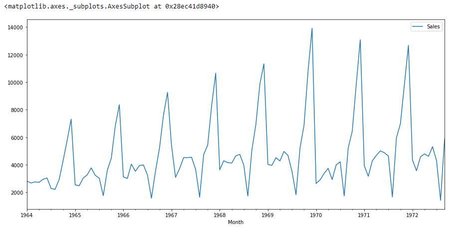
if we look at the graph above then we can find a trend that there is a time when sales are high and vice versa. That means we can see that the data follows seasonality.. For ARIMA, the first thing we do is identify if the data is stationary or non-stationary. if the data is not stationary, we will try to make them stationary and then process more.
Let us check that if the given data set is stationary or not, for that we use adfuller.
from statsmodels.tsa.stattools import adfuller
I have imported the adfuller by running the above code.
test_result=adfuller(df['Sales'])
To identify the nature of the data, we will use the null hypothesis.
H0: The null hypothesis: It is a statement about the population that is believed to be true or used to make an argument unless it can be shown to be incorrect beyond a reasonable doubt.
H1: The alternative hypothesis: It is a statement about the population that contradicts H0 and what we conclude when we reject H0.
#Ho: it is not stationary
# H1: is stopped
We will consider the null hypothesis that the data are not stationary and the alternative hypothesis that the data are stationary.
def adfuller_test(sales):
    result=adfuller(sales)
    labels = ['ADF Test Statistic','p-value','#Lags Used','Number of Observations']
    for value,label in zip(result,labels):
        print(label+' : '+str(value) )

if result[1] <= 0.05:
    print("strong evidence against the null hypothesis(Ho), reject the null hypothesis. Data is stationary")
else:
    print("weak evidence against null hypothesis,indicating it is non-stationary ")

adfuller_test(df['Sales'])
After running the above code we will get the value P,
ADF Test Statistic : -1.8335930563276237
p-value : 0.3639157716602447
#Lags Used : 11
Number of Observations : 93
Here the value P is 0.36, which is greater than 0.05, which means that the data accepts the null hypothesis, which means that the data is not stationary.
Let's try to see the first difference and the seasonal difference:
df['Sales First Difference'] = df['Sales'] - df['Sales'].shift(1)
df['Seasonal First Difference']=df['Sales']-df['Sales'].shift(12)
df.head()

# Again testing if data is stationary
adfuller_test(df['Seasonal First Difference'].drop())
ADF Test Statistic : -7.626619157213163
p-value : 2.060579696813685e-11
#Lags Used : 0
Number of Observations : 92
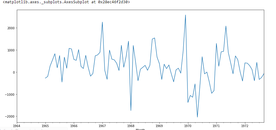
Here the value P is 2.06, which means that we will reject the null hypothesis. Then the data is stationary.
df['Seasonal First Difference'].plot()
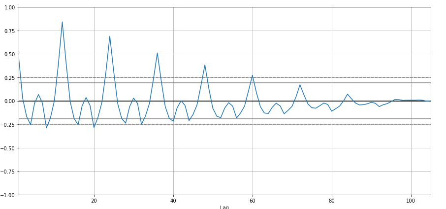
I'm going to create autocorrelation:
from pandas.plotting import autocorrelation_plot
autocorrelation_plot(df['Sales'])
plt.show()
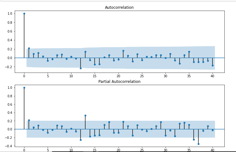
from statsmodels.graphics.tsaplots import plot_acf,plot_pacf
import statsmodels.api as sm
fig = plt.figure(figsize=(12,8))
ax1 = fig.add_subplot(211)
fig = sm.graphics.tsa.plot_acf(df['Seasonal First Difference'].drop(),lags=40,ax=ax1)
ax2 = fig.add_subplot(212)
fig = sm.graphics.tsa.plot_pacf(df['Seasonal First Difference'].drop(),lags=40,ax=ax2)
# For non-seasonal data
#p=1, d=1, q=0 or 1

from statsmodels.tsa.arima_model import ARIMA
model=ARIMA(df['Sales'],order=(1,1,1))
model_fit=model.fit()
model_fit.summary()
| Dep. Variable: | D. Sales | No. Observations: | 104 |
|---|---|---|---|
| Model: | ARIMA (1, 1, 1) | Logarithmic probability | -951.126 |
| Method: | css-mle | SD de innovaciones | 2227.262 |
| Date: | Mié, 28 oct 2020 | AIC | 1910.251 |
| Weather: | 11:49:08 | BIC | 1920.829 |
| Shows: | 02-01-1964 | HQIC | 1914.536 |
| – 09-01-1972 |
| coef | std err | With | P> | With | | [0.025 | 0.975] | |
|---|---|---|---|---|---|---|
| constant | 22.7845 | 12.405 | 1.837 | 0.066 | -1.529 | 47.098 |
| ar. L1. D.Sales | 0.4343 | 0,089 | 4.866 | 0.000 | 0,259 | 0,609 |
| ma. L1. D.Sales | -1,0000 | 0,026 | -38.503 | 0.000 | -1.051 | -0,949 |
| True | Imaginario | Module | Frequency | |
|---|---|---|---|---|
| AR.1 | 2.3023 | + 0,0000j | 2.3023 | 0,0000 |
| MA.1 | 1,0000 | + 0,0000j | 1,0000 | 0,0000 |
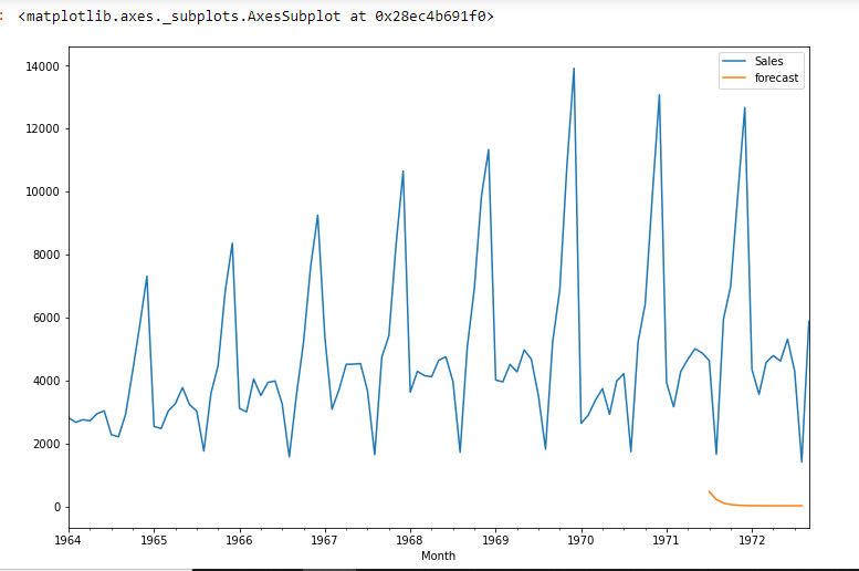
df['forecast']=model_fit.predict(start=90,end=103,dynamic=True)
df[['Sales','forecast']].plot(figsize=(12,8))
import statsmodels.api as sm
model=sm.tsa.statespace.SARIMAX(df['Sales'],order=(1, 1, 1),seasonal_order=(1,1,1,12))
results=model.fit()
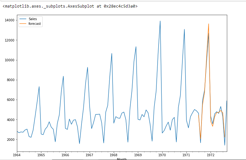
df['forecast']=results.predict(start=90,end=103,dynamic=True)
df[['Sales','forecast']].plot(figsize=(12,8))
from pandas.tseries.offsets import DateOffset
future_dates=[df.index[-1]+ DateOffset(months=x)for x in range(0,24)]
future_datest_df=pd. DataFrame(index=future_dates[1:],columns=df.columns)
future_datest_df.tail()
future_df=pd.concat([df,future_datest_df])
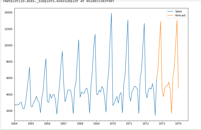
future_df['forecast'] = results.predict(start = 104, end = 120, dynamic= True)
future_df[['Sales', 'forecast']].plot(figsize=(12, 8))
Conclution
Time series forecasting is really useful when we have to make future decisions or we have to do analysis, we can do it quickly using ARIMA, there are many other models from which we can do time series forecasting, but ARIMA is really easy to understand.
Hope this article helps you and saves you a good amount of time.. Let me know if you have any suggestions..
HAPPY CODING.
Prabhat Pathak (Linkedin profile) is a senior analyst.


