This article was published as part of the Data Science Blogathon.
Understand the problem of overfitting in decision trees and solve it by pruning complexity and minimal cost using Scikit-Learn in Python
Decision Tree is one of the most intuitive and effective tools in a data scientist's toolkit.. It has an inverted tree structure that was once used only in decision analysis, but now it's also a brilliant machine learning algorithm, especially when we have a sorting problem on our hands.
These decision trees are well known for their ability to capture patterns in the data.. But, excess of anything is harmful, truth? Decision trees are infamous as they can get too clinging to the data they are trained on.
Therefore, our tree gives poor implementation results because it can't deal with a new set of values.

But do not worry! Like a skilled mechanic he has wrenches of all sizes available in his toolbox, an expert data scientist also has his set of techniques to deal with any kind of problem. And that is what we will explore in this article..
The role of pruning in decision trees
Pruning is one of the techniques used to overcome our overfitting problem. Pruning, in its literal sense, is a practice that involves the selective removal of certain parts of a tree (the plant), like branches, shoots or roots, to improve tree structure and promote healthy growth. This is exactly what pruning also does with our decision trees. It makes it versatile so that it can adapt if we give it some kind of new information, thus solving the problem of overfitting.
Reduce the size of a decision tree, which may slightly increase the error of trainingTraining is a systematic process designed to improve skills, physical knowledge or abilities. It is applied in various areas, like sport, Education and professional development. An effective training program includes goal planning, regular practice and evaluation of progress. Adaptation to individual needs and motivation are key factors in achieving successful and sustainable results in any discipline...., but drastically decrease the test error, what makes it more adaptable.
Pruning of minimal cost and complexity is one of the types of decision tree pruning.
This algorithm is parameterized by α (≥0) known as the complexity parameter.
The complexity parameter is used to define the cost-complexity measure, Ra(T) of a given tree T: Ra(T) = R (T) + a | T |
where | T | is the number of terminal nodes in T and R (T) is traditionally defined as the total misclassification rate of the terminal nodes.
In its version 0.22, Scikit-learn introduced this parameter called ccp_alpha (Yes! It is short for Cost complexity pruning – Alfa) to decision trees that can be used to do the same.
Building the decision tree in Python
We will use the Iris dataset to fit the decision tree. You can download the dataset here.
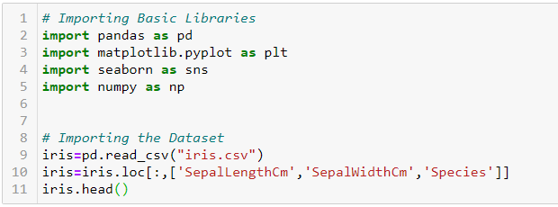
First, let's import the required basic libraries and dataset:
The dataset looks like this:
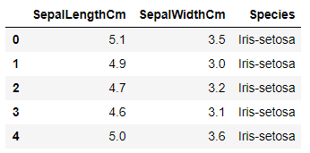
Our goal is to predict the species of a flower based on the length and width of its sepal.
We will divide the data set into two parts: train and test. We are doing this so that we can see how our model works also on invisible data. We will use the train_test_split function of sklearn.model_selection to divide the data set.

Now, let's fit a decision tree to the part of the train and predict both in the test and in the training. we will use DecisionTreeClassifier of sklearn.tree for this purpose.
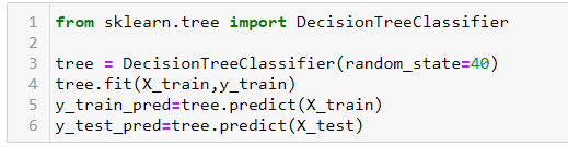
By default, the decision tree function does not do any pruning and allows the tree to grow as much as it can. We obtain an accuracy score of 0,95 Y 0,63 on the train and on the test piece, respectively, as it's shown in the following. We can say that our model is overfitted, namely, memorizing the part of the train, but it may not work equally well in the test part.

Decision tree in sklearn it has a function called cost_complexity_pruning_path, which gives the effective alphas of the subtrees during pruning and also the corresponding impurities. In other words, we can use these alpha values to prune our decision tree:
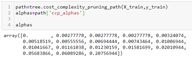
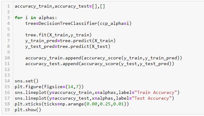
We will set these alpha values and pass them to the ccp_alpha parameter of our DecisionTreeClassifier. Looping over it alfas headquarters, we will find the precision in the training and testing parts of our data set.
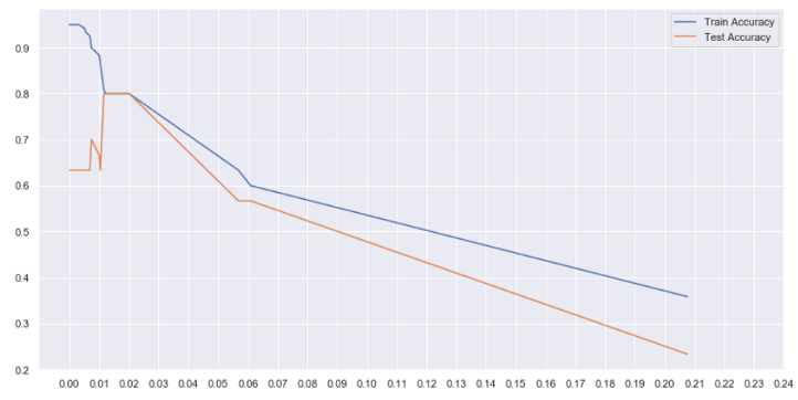
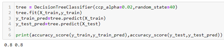
In the graph above, we can see that between alpha = 0.01 Y 0.02, we obtain the highest test precision. Although the accuracy of our train has decreased to 0,8, our model is now more generalized and will work better with invisible data.