Data Visualization Guide for SAS

Introduction

A picture is worth a thousand words!

In today's competitive environment, companies want a faster decision-making process, ensuring they stay ahead of the race.

Data visualization aids in two critical stages in the data-driven decision process (Like shown in the next figure):

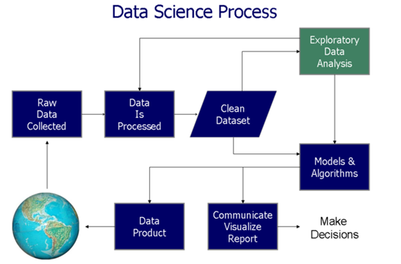
In this article, we will explore the 4 data visualization applications and their implementation in SAS. For a better understanding, we have taken sample data sets to create this visualization. Then, the main aspects of data visualization are shown:

1. Making comparison: Includes bar chart, line graph, bar line graph, column chart, clustered bar column chart.
2. Study relationship: Includes bubble chart, scatter plot
3. Studying Distribution: Includes histogram, Dispersion diagram,
4. Understand composition: Includes stacked column chart

Let us begin!

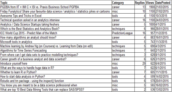
For illustration purposes, we will use a data set 'to discuss’ taken from the Analytical Vidhya Discuss. The data contains the topic of discussion, the category, the number of responses to the post and the total number of Views. The data contains the 20 main topics:

1. Making a comparison

a) Bar graphic

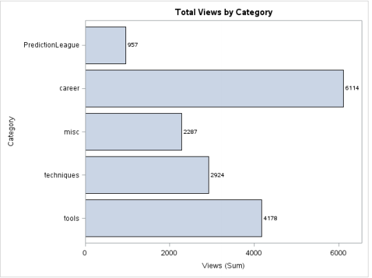
A bar graphic, also know as bar graphic represents grouped data using rectangular bars with lengths proportional to the values ​​they represent. Bars can be drawn vertically or horizontally. A vertical bar chart is sometimes called a column bar chart.

Illustration

Target: We want to know the number of views of each category represented graphically through a bar graph.

Code:

proc sgplot data = discuss;
     hbar category/response = views stat = sum
                           datalabel datalabelattrs=(weight=bold);
     title 'Total Views by Category';
run;       

Production:

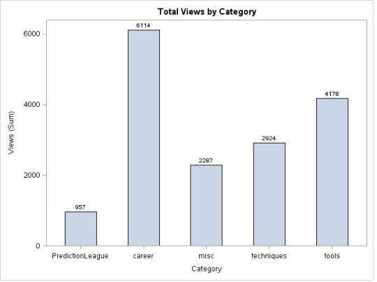
B) Column chart

Column charts are often self explanatory. They are simply the vertical version of a bar graph where the length of the bars is equal to the magnitude of the value they represent. Here is a maneuver: turn the graph shown above into -90 degrees, will become a column chart.

Code:

proc sgplot data = discuss;
     hbar category/response = views stat = sum
                    datalabel datalabelattrs=(weight=bold) barwidth = 0.5; /* Assign width to bars*/
    title 'Total Views by Category';
run;

Production:

-> Explanation of the code for the bar chart and column chart:

• Category: the variable according to which the data should be grouped.
• Response = views: statistics specified by stat = option are calculated for variable views grouped by category variable.
• The Datalabel option specifies that we want the calculated values ​​to be displayed for each bar.
• The Weight = bold option specifies that the data labels for each bar will be displayed in bold.
• The bar width option is used to assign width to the bars. The default is 0.8 and the range is 0.1-1.

c) Bar graphic / clustered column chart

This type of representation is useful when we want to visualize the distribution of data in two categories.

Target: We want to analyze the total views of the topics in the discussion forum by category and publication date.

Code:

data discuss_date;
set discuss;
month = month(DatePosted);
month_name=PUT(DatePosted,monname.);
  put month_name= @;
run;
proc sgplot data=discuss_date;
    vbar category/ response=views group=month_name groupdisplay=cluster
                 datalabel datalabelattrs = (weight = bold) dataskin=gloss; yaxis grid;
run;

Production:

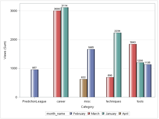
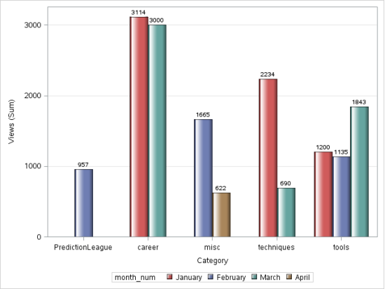
But nevertheless, there is a problem with this image, the months are not in chronological order. To solve this, we use PROC FORMAT.

Code with PROC FORMAT:

data discuss_date;
set discuss;
month = month(DatePosted);
month_num = input(month,5.);
run;

PROC FORMAT;
   VALUE monthfmt
        1 = 'January'
        2 = 'February'
        3 = 'March' 
        4 = 'April';
RUN;

proc sgplot data=discuss_date;
  vbar category/ response=views group = month_num groupdisplay=cluster datalabel 
                    datalabelattrs = (weight = bold) dataskin=gloss grouporder= ascending;
   format month_num monthfmt.;
  yaxis grid;
run;

Production:

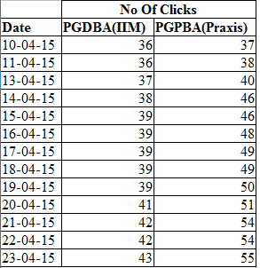
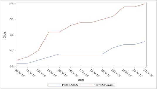
D) Line graph

A Line graph O line graph is a type of graph that displays information as a series of data points called “bookmarks” connected by straight line segments. A line chart is often used to visualize trends in data over time intervals., a time series, so the line is often drawn chronologically. In these cases they are known as run graphics.

For this illustration, we will use data from PGDBA from IIT + IIM C + ISI frente a Praxis Business School PGPBA.

Code:

proc sgplot data = clicks;
     vline date/response = PGDBA_IIM_ ;
     vline date/response = PGPBA_Praxis_;
     yaxis label = "Clicks";
run;

Production:

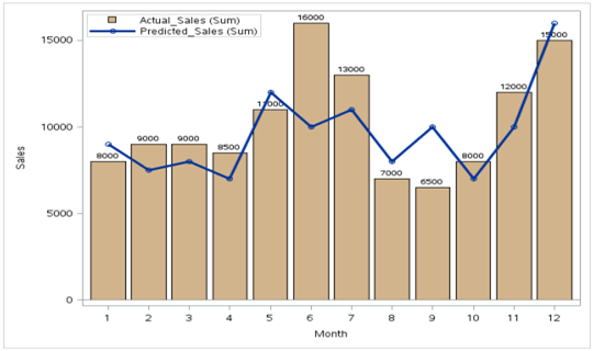
e) Bar line chart

This combination chart combines the features of the bar chart and the line chart. Displays the data using a series of bars and / or lines, each of which represents a particular category. A combination of bars and lines in the same visualization can be useful when comparing values ​​in different categories.

Target: We want to compare projected sales with actual sales for different time periods.

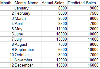
Code:

proc sgplot data=barline;
  vbar month/ response=actual_sales datalabel datalabelattrs = (weight = bold)
                   fillattrs = (color = tan);
  vline month/ response=predicted_sales
                 lineattrs =(thickness = 3) markers;
  xaxis label= "Month";
  yaxis label = "Sales";
  keylegend / location=inside position=topleft across=1;
  run;

Note: The data must be ordered by the x-axis variable.

Production:

2) Study the relationship

a) Bubble chart

A bubble chart is a type of chart that displays three dimensions of data. Each entity with its triplet (v₁, v₂, v₃) associated data is plotted as a disk expressing two of the v_I values ​​across disk xy location and the third for its size. – Source: Wikipedia.

Data for OS:

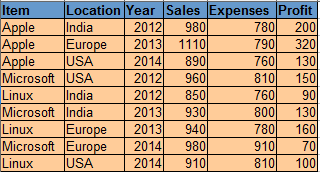
Code:

proc sgplot data = os;
     bubble X=expenses Y=sales size= profit
     /fillattrs=(color = teal) datalabel = Location;
run;

Production:

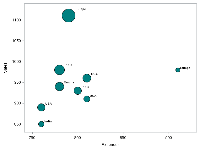
As we can see, there is a record for which Sales and Profits are highest while comparative expenses are less than some other data points.

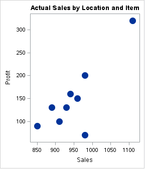
b) Scatter plot for the relationship

A simple scatter diagram between two variables can give us an idea about the relationship between them: lineal, exponential, etc. This information can be useful during a later analysis.

Code:

proc sgplot data = os;
    title 'Relationship of Profit with Sales';
    scatter X= sales Y = profit/
                     markerattrs=(symbol=circlefilled size=15);
run;

Production:

3. Study the distribution

a) Histogram

A histogram is a graphical representation of the distribution of numerical data. It is an estimate of the probability distribution of a continuous variable. To construct a histogram, the first step is “Group” the range of values, namely, divide the entire range of values ​​into a series of small intervals and then count how many values ​​fall in each interval. Bins are generally specified as consecutive intervals, non-overlapping of a variable. The containers (intervals) must be adjacent and, as usual, the same size. The rectangles in a histogram are drawn so that they touch each other to indicate that the original variable is continuous.

Code:

proc sgplot data = sashelp.cars;
     histogram msrp/fillattrs=(color = steel)scale = proportion;
     density msrp;
run;

Production:

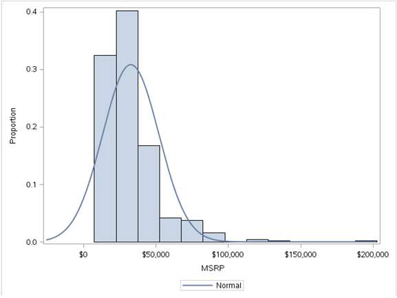
We have used the sashelp.mtcars dataset here. A histogram of the MSRP variable gives us the previous figure. This tells us that the MSRP variable is skewed to the right, indicating that most of the data points are below $ 50,000. Meaningful insights can be found from histograms.

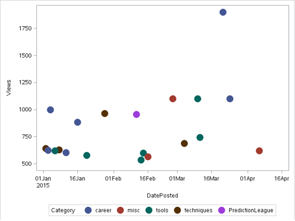
b) Dispersion diagram

in a scatter plot data is displayed as a collection of points, each with the value of one variable that determines the position on the horizontal axis and the value of the other variable that determines the position on the vertical axis. It can be used both to see the distribution of data. and access the relationship between variables.

Note: for illustration, we will use a data set 'to discuss’ taken from the Analytical Vidhya Discuss

Code:

proc sgplot data = discuss;
     scatter X= dateposted Y = views/group=category
                    markerattrs=(symbol=circlefilled size=15);
run;

Production:

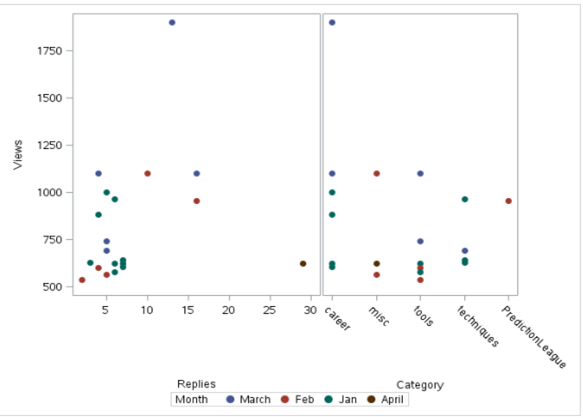
the SGSCATTER The procedure can also be used for scatter plots. It has the advantage of being able to produce multiple scatter diagrams. Below is the output using sgcscatter:

Code:

proc sgscatter data = discuss;
     compare y = views  x = (replies category)
               /group = month markerattrs=(symbol = circlefilled size = 10);
run;

Production:

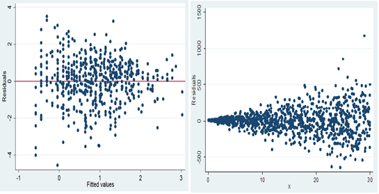
An important use of the scatter plot is the interpretation of the residuals from the linear regression. A scatterplot of the residuals versus the predicted values ​​of the predicted variable helps us determine whether the data are heteroscedastic or homoscedastic..

HETEROSQUEDASTIC HOMOSQUEDASTIC

4) Composition

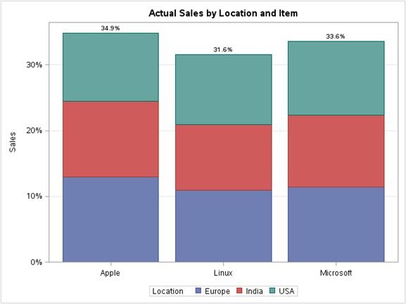
a) Stacked column chart:

On a stacked bar chart, stacked bars represent different groups on top of each other. The height of the resulting bar shows the combined result of the groups.

For instance, if we want to see the total sales per item grouped by location in the total data of the operating system dataset, we can use the stacked column chart. Below is the illustration:

Code:

proc sgplot data = os;
  title 'Actual Sales by Location and Item';
  vbar Item / response=Sales group=Location stat=percent datalabel;
  xaxis display=(nolabel);
  yaxis grid  label="Sales";
run;

Production:

Final notes:

Visualizations become a natural way to understand bulk data. They convey information in a simple way and facilitate the exchange of ideas with others. In this article, we analyze some basic visualizations that can be made through SAS base. These can be a great way to summarize our data, get information, find relationships, etc.

Did you find this article useful? Is there any other visualization you have used that you can share with our audience? Feel free to share them through the comments below..

If you like what you have just read and want to continue learning about analytics, subscribe to our emails, Follow us on twitter or like ours page the Facebook.

Related