This article was published as part of the Data Science Blogathon.
Introduction
Time series anomaly detection
The entire anomaly detection process for a time series is carried out in 3 Steps:
- Decompose the time series into the underlying variables; Trend, seasonality, residue.
- Create upper and lower thresholds with some threshold value
- Identify data points that are outside the thresholds as anomalies.
Case study
Let's download the dataset from the Singapore government website which is easily accessible. Total electricity consumption in households by type of dwelling. Singapore Government Data Website Crashes Quite Easily. This data set shows the total electricity consumption of households by type of dwelling (and GWh).
Managed by the Energy Market Authority
Annual Frequency
Source (s) Energy Market Authority
Singapore Open Data License License
Install and upload R packages
In this exercise, we will work with 2 Key Packages for Time Series Anomaly Detection in R: anomalous Y timetk. These require that the object be created as a tibble of time, so we will also load the tibble packages. Let's first install and load these libraries.
pkg <- c('tidyverse','tibbletime','anomalize','timetk')
install.packages(pkg)
library(tidyverse)
library(tibbletime)
library(anomalize)
library(timetk)
Load data
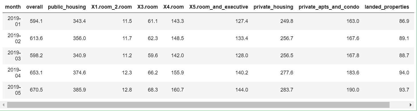
In the previous step, we have downloaded the file of total electricity consumption by type of home (and GWh) from the Singapore Government website. Let's load the CSV file into an R data frame.
df <- read.csv("C:Anomaly Detection in Rtotal-household-electricity-consumption.csv")
head(df,5)
Data processing
Before we can apply any anomaly algorithm to the data, we have to change it to a date format.
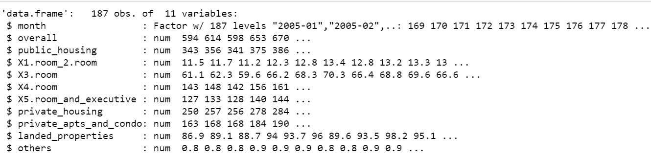
The column ‘month’ is originally in factorial format with many levels. Let us convert it to a date type and select only the relevant columns in the data frame.
str(df)
# Change Factor to Date format
df$month <- paste(df$month, "01", sep="-")
# Select only relevant columns in a new dataframe
df$month <- as.Date(df$month,format="%Y-%m-%d")
df <- df %>% select(month,overall)
# Convert df to a tibble
df <- as_tibble(df)
class(df)
Using the ‘anomalize package’
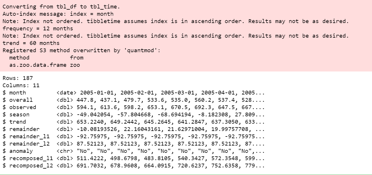
The R package ‘anomalize’ enables a workflow to detect data anomalies. The main functions are time_decompose (), anomaly (), Y time_recompose ().
df_anomalized <- df %>%
    time_decompose(overall, merge = TRUE) %>%
    anomalize(remainder) %>%
    time_recompose()
df_anomalized %>% glimpse()
View anomalies
We can then visualize the anomalies using the plot_anomalies () function.
df_anomalized %>% plot_anomalies(ncol = 3, alpha_dots = 0.75)

Trend and seasonality adjustment
With anomalize, it's easy to make adjustments because everything is done with a date or timestamp information, so you can intuitively select increments for time periods that make sense (for instance, "5 minutes" or "1 month").
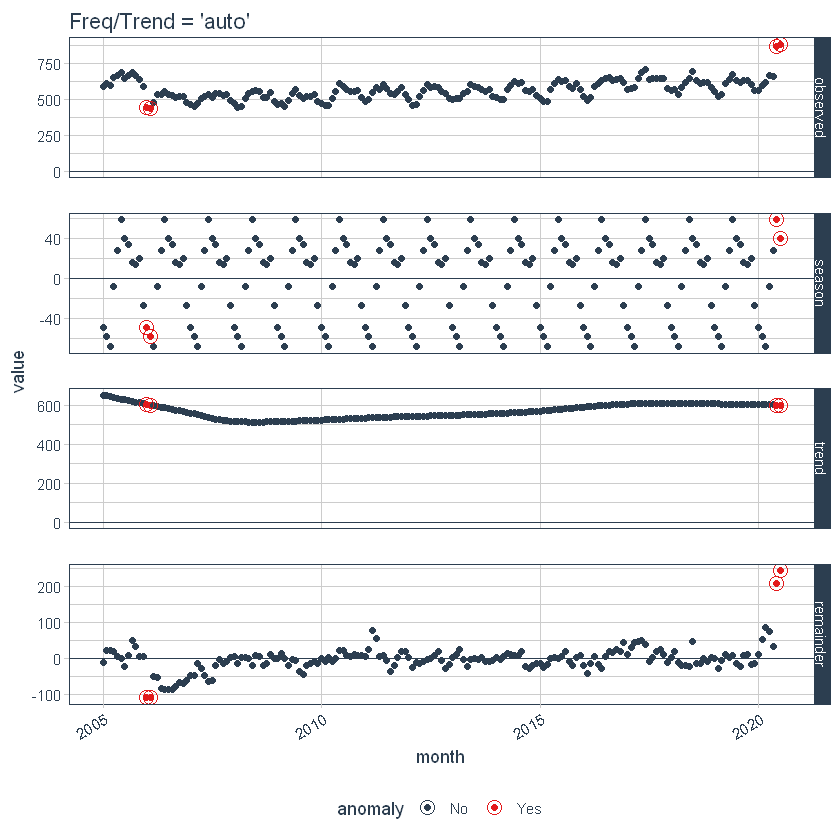
First, note that a frequency and a trend were automatically selected for us. This is by design. The arguments frequency = “auto” and trend = “auto” are the default values. We can visualize this decomposition using plot_anomaly_decomposition ().
p1 <- df_anomalized %>%
    plot_anomaly_decomposition() +
    ggtitle("Freq/Trend = 'auto'")
p1

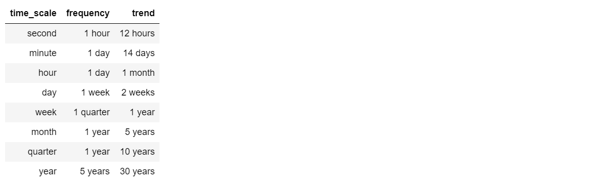
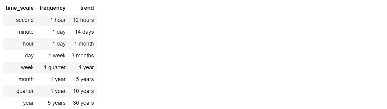
When it's used “auto”, get_time_scale_template () used to determine the logical frequency and trend intervals based on the scale of the data. You can discover the logic:
get_time_scale_template()
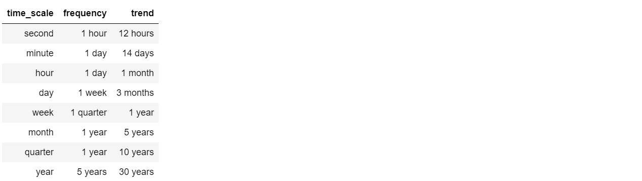
This implies that if the scale is 1 day (which means that the difference between each data point is 1 day), then the frequency will be 7 days (O 1 week) and the trend will be around 90 days (O 3 months). This logic can be easily adjusted in two ways: local parameter setting and global parameter setting.
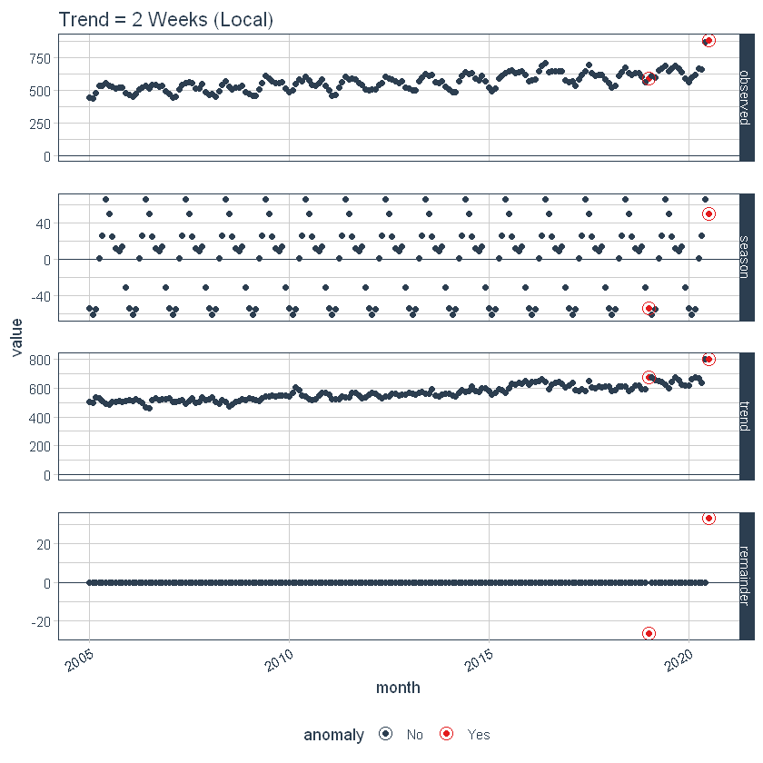
Setting the local parameters
The adjustment of the local parameters is carried out by adjusting the parameters according to. Then, we adjust the trend = “2 weeks”, which makes for a pretty overfitting trend.
p2 <- df %>%
    time_decompose(overall,
                   frequency = "auto",
                   trend     = "2 weeks") %>%
    anomalize(remainder) %>%
    plot_anomaly_decomposition() +
    ggtitle("Trend = 2 Weeks (Local)")
# Show plots
p1
p2
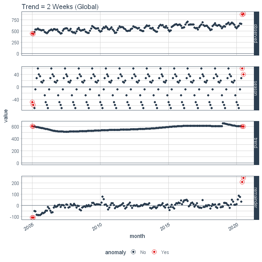
Global parameter setting
We can also adjust globally using set_time_scale_template () to update the default template to one we prefer. We will change the trend from “3 months” a “2 weeks” for the time scale = “day”. Use time_scale_template () to retrieve the timeline template with which the anomaly begins, mute () the trend field at the desired location and use set_time_scale_template () to update the template in global options. We can retrieve the updated template using get_time_scale_template () to verify that the change has been executed correctly.
time_scale_template() %>%
    mutate(trend = ifelse(time_scale == "day", "2 weeks", trend)) %>%
    set_time_scale_template()
get_time_scale_template()
Finally, we can rerun the time_decompose () with default values, and we can see that the trend is "2 weeks".
p3 <- df %>%
    time_decompose(overall) %>%
    anomalize(remainder) %>%
    plot_anomaly_decomposition() +
    ggtitle("Trend = 2 Weeks (Global)")
p3
Let's reset the timeline template defaults to the original defaults.
time_scale_template() %>%
    set_time_scale_template()
# Verify the change
get_time_scale_template()
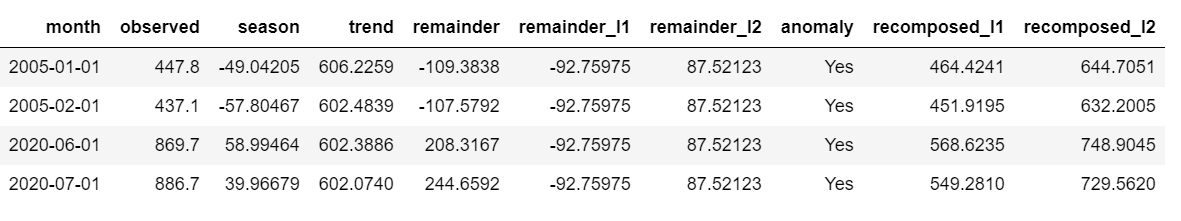
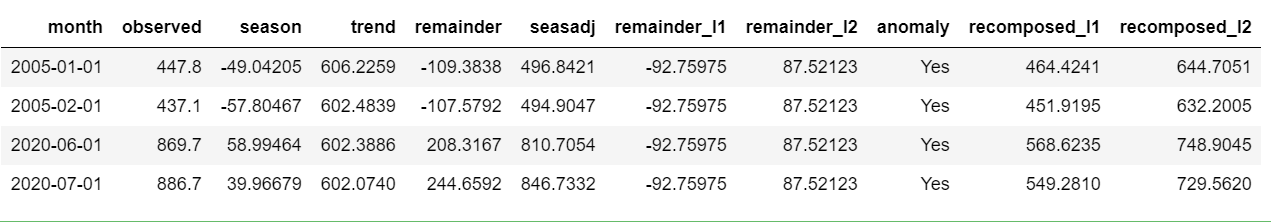
Extract the anomalous data points
Now, we can extract the actual data points that are anomalies. For that, you can run the following code.
df %>%
  time_decompose(overall) %>%
  anomalize(remainder) %>%
  time_recompose() %>%
  filter(anomaly == 'Yes')
Adjusting Alpha and Max Anoms
the alfa Y max_anoms are the two parameters that control the anomaly () function. H
Alfa
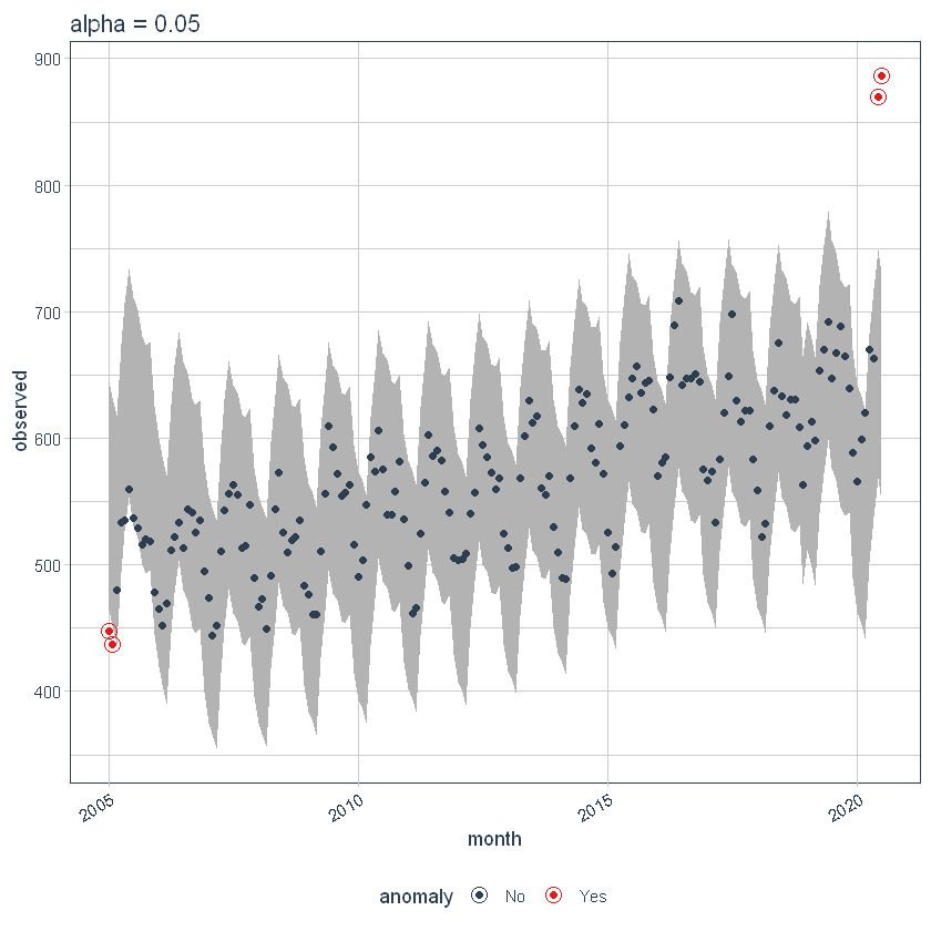
We can adjust the alpha, which is configured in 0.05 default. By default, the bands only cover the outside of the range.
p4 <- df %>%
    time_decompose(overall) %>%
    anomalize(remainder, alpha = 0.05, max_anoms = 0.2) %>%
    time_recompose() %>%
    plot_anomalies(time_recomposed = TRUE) +
    ggtitle("alpha = 0.05")
#> frequency = 7 days
#> trend = 91 days
p4
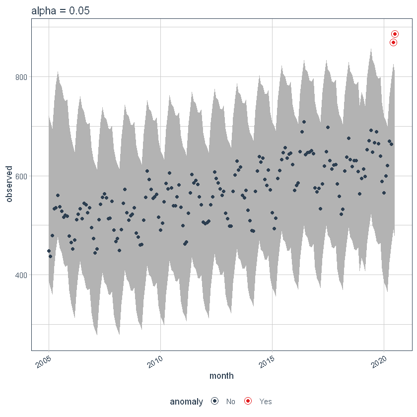
If we decrease the alpha, increase the bands, what makes it harder to be an outlier. Here, you can see the bands have gotten twice as big.
p5 <- df %>%
    time_decompose(overall) %>%
    anomalize(remainder, alpha = 0.025, max_anoms = 0.2) %>%
    time_recompose() %>%
    plot_anomalies(time_recomposed = TRUE) +
    ggtitle("alpha = 0.05")
#> frequency = 7 days
#> trend = 91 days
p5
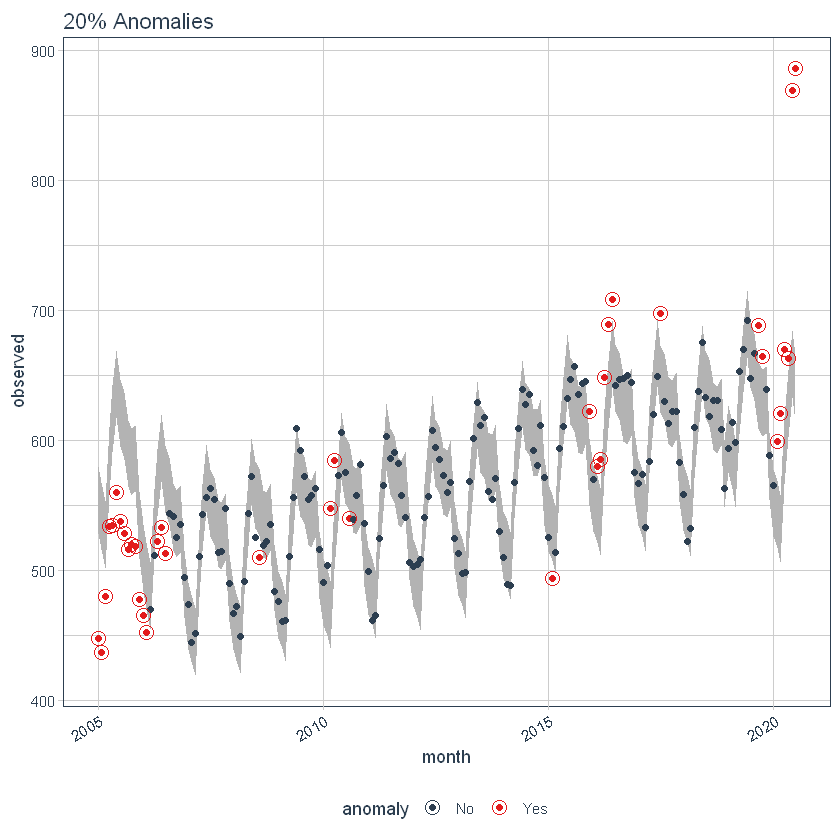
Max Anoms
the max_anoms The parameter is used to control the maximum percentage of data that can be an anomaly. Let's set alpha = 0.3 so that pretty much anything is an outlier. Now let's try a comparison between max_anoms = 0.2 (20% allowed anomalies) y max_anoms = 0.05 (5% allowed anomalies).
p6 <- df %>%
time_decompose(overall) %>%
anomalize(remainder, alpha = 0.3, max_anoms = 0.2) %>%
time_recompose() %>%
plot_anomalies(time_recomposed = TRUE) +
ggtitle("20% Anomalies")
#> frequency = 7 days
#> trend = 91 days
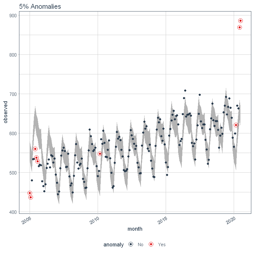
p7 <- df %>%
time_decompose(overall) %>%
anomalize(remainder, alpha = 0.3, max_anoms = 0.05) %>%
time_recompose() %>%
plot_anomalies(time_recomposed = TRUE) +
ggtitle("5% Anomalies")
#> frequency = 7 days
#> trend = 91 days
p6
p7
Using the 'timetk package’
It is a toolkit for working with time series in R, to trace, discuss and present engineer time series data to perform machine learning predictions and predictions.
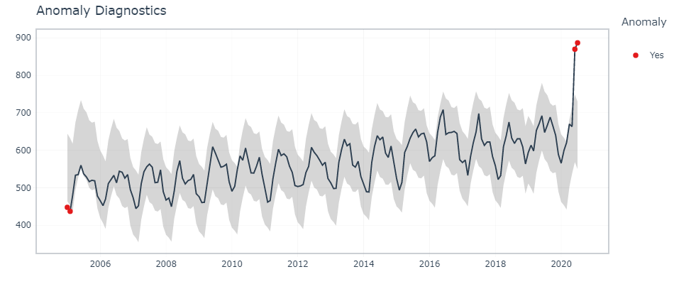
Interactive viewing of anomalies
Here, timetk’s The plot_anomaly_diagnostics function () allows you to modify some of the parameters on the fly.
df %>% timetk::plot_anomaly_diagnostics(month,overall, .facet_ncol = 2)
Interactive anomaly detection
To find the exact data points that are anomalies, we use tk_anomaly_diagnostics () function.
df %>% timetk::tk_anomaly_diagnostics(month, overall) %>% filter(anomaly=='Yes')
Conclution
In this article, we have seen some of the popular packages in R that can be used to identify and visualize anomalies in a time series. To provide some clarity on anomaly detection techniques in R, we did a case study on a publicly available data set. There are other methods to detect outliers and can also be explored.


