Overview
- Microsoft Excel is one of the most used tools for data analysis.
- Learn about essential Excel functions used to analyze data for business analysis.
- Data analysis with Excel serves as a precursor to data science with R or Python
* This article was originally published on 2015 and was updated in April 2020.
Introduction
I have always admired the immense power of Standing out. This software is not only capable of basic data calculations, but you can also perform data analysis using it. It is widely used for many purposes, including financial modeling and business planning. It can become a good stepping stone for people who are new to the world of business analytics..
Included before learning Python, it is advisable to have knowledge of Excel. It doesn't hurt to add Excel to your skill set. Excel, with its wide range of functions, visualizations and matrices, allows you to quickly generate insights from data that would be difficult to see otherwise. And this is a crucial aspect of any business analysis project..
In fact, we have designed a the entire comprehensive Business Analytics program for you, With Excel as a key component! Be sure to check it out and give yourself the gift of a career in business analytics..
I feel lucky that my journey started with Excel. Over the years, I have learned many tricks to work with data faster than ever. Excel has many functions. Sometimes it gets confusing to choose the best.
In this article, I will provide you with some tips and tricks to work in Excel and save you time. This article is best suited for people interested in updating their data analysis skills.

Commonly used functions
1. Vlookup (): Helps to find a value in a table and returns a corresponding value. Let's see the table below (Policy and Client). In the policy table, we want to map the city name of the customer tables based on the common key “Client ID”. Here, the vlookup function () would help to perform this task.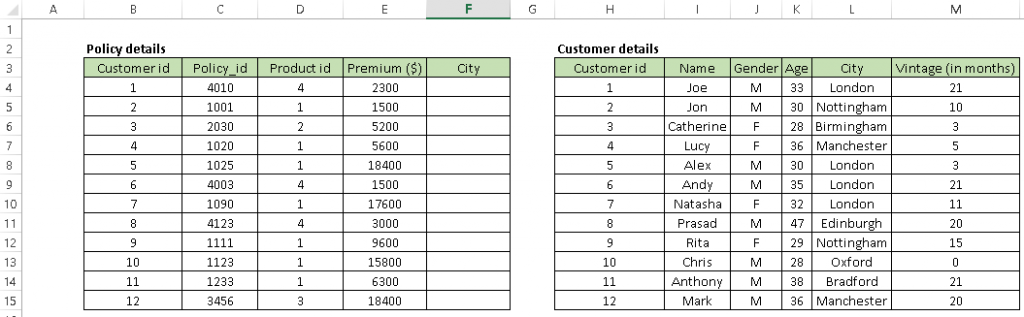
Syntax: =VLOOKUP(Key to lookup, Source_table, column of source table, are you ok with relative match?)
For the above problem, we can write the formula in the cell “F4” as = VLOOKUP (B4, $ H $ 4: $ L $ 15, 5, 0) and this will return the city name for all customer IDs 1 and it will post that copy this formula for all customer IDs.
Tip: Don't forget to lock the range of the second table with a sign “$”, a common mistake when copying this formula. This is known as a relative reference..
2. CONCATENAR (): It is very useful to combine text from two or more cells into one. For instance, we want to create url based on input of hostname and request path.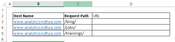
Syntax: =Concatenate(Text1, Text2,.....Textn)
The above problem can be solved using the formula, = concatenar (B3, C3) and copy it.
Tip: I prefer to use the symbol “&”, because it is shorter than writing a formula of “concatenar” complete, and does exactly the same. The formula can be written as “= B3 & C3”.
3. LEN () – This function informs you about the length of a cell, namely, the number of characters, including spaces and special characters.
Syntax: = Len(Text)
Example: = Len (B3) = 23
4. INFERIOR (), SUPERIOR () and SUITABLE () –These three functions help to change the text to upper case, lower case and sentences respectively (First letter of each word capitalized).
Syntax: =Upper(Text)/ Lower(Text) / Proper(Text)
In a data analysis project, these are useful for converting classes from a different case into a single case, on the contrary, different classes of the given characteristic are considered. Look at the snapshot below, column A has five classes (labels) while column B has only two because we have converted the content to lowercase.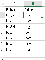
5. TRIM (): This is a useful function used to clean up text that has leading and trailing whitespace. Often, when you get a data dump from a database, the text you are dealing with is padded with blanks. And if you don't take care of them, they are also treated as single entries in a list, which is certainly not useful.
Syntax: =Trim(Text)
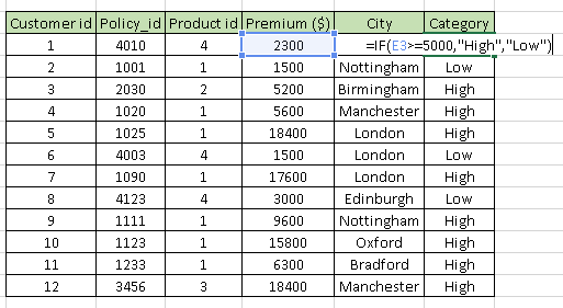
6. AND (): I find it one of the most useful functions in Excel. It allows you to use conditional formulas that calculate in one way when a certain thing is true and in another way when it is false. For instance, you want to mark each sale as “High” Y “Baja”. If sales are greater than or equal to $ 5000, then “Alto” O “Low”.
Syntax: =IF(condition, True Statement, False Statement)
Generating inference from data
1. Dynamic table: Whenever you work with company data, look for answers to questions like “How much revenue do the branches in the northern region bring??” O “What was the average number of customers for product A?” and many others.
Excel pivot table helps you answer these questions effortlessly. A pivot table is a summary table that allows you to count, average, add and perform other calculations according to the reference function you have selected, namely, converts a data table into an inference table that helps us make decisions. Look at the snapshot below: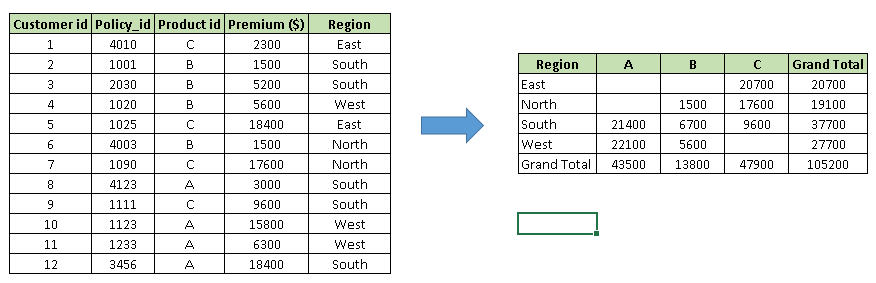 Above, you can see the table on the left has sales details for each customer with region and product mapping. In the table on the right, We have summarized the information at the region level that now helps us to generate an inference that the South region has the highest sales.
Methods for creating a pivot table:
Paso 1: Click somewhere in the data list. Choose the Insert tab and click Dynamic table. Excel will automatically select the area containing the data, including headers. If you don't select the area correctly, drag over the area to select it manually. It is best to place the pivot table on a new sheet, so click New worksheet for the location and then click OK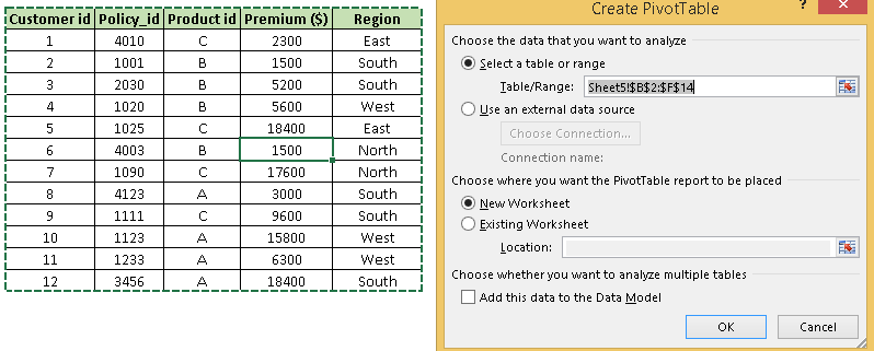 Paso 2: Now, you can see the Field List pane of the pivot table, containing the fields of your list; all you need to do is place them in the boxes at the bottom of the panel. Once i have done that, the diagram on the left becomes your pivot table.
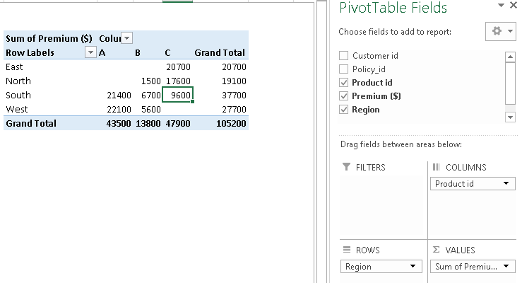 Above, you can see we have organized “Region” In line, “Product ID“In column and sum of”Before”It is taken as value. Now you are ready with the pivot table showing the sum of the premium by region and product. You can also use count, average, minimum, maximum and other summary metrics.
2. Chart Creation: Create a box / chart in Excel requires nothing more than selecting the data range you want to plot and pressing F11. This will create an Excel chart with the default chart style, but you can change it by selecting a different chart style. If you prefer the chart to be on the same worksheet as the data, instead of pressing F11, press ALT + F1.
Of course, in any case, once you have created the chart, you can customize it to your particular needs to communicate the desired message.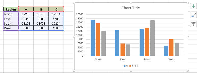
Data cleansing
1. Remove duplicate values: Excel has a built-in function to remove duplicate values from a table. Remove duplicate values from given table based on selected columns, namely, if you have selected two columns, looks for a duplicate value that has the same combination of data from both columns.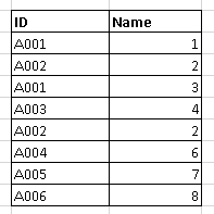
Above, you can see that A001 and A002 have duplicate value, but if we select both columns “ID” Y “Name”, So we only have a duplicate value (A002, 2).
Follow these steps to remove duplicate values: Select data -> Go to the Data ribbon -> Remove duplicates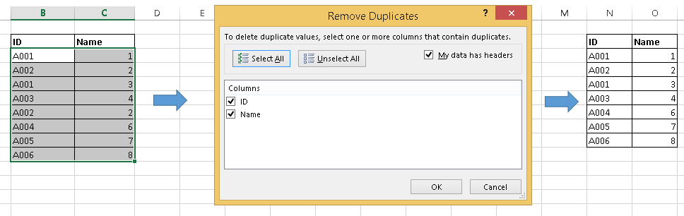
2. Text to columns: Suppose you have data stored in the column as shown in the following snapshot.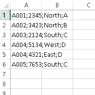 Above, you can see that the values are separated by semicolons “;”. Now, to split these values into a different column, I will recommend using the “Text to columns”Feature in Excel. Follow the steps below to convert it to different columns:
- Select range A1: A6
- Go to the tape “Data” -> “Text to columns”
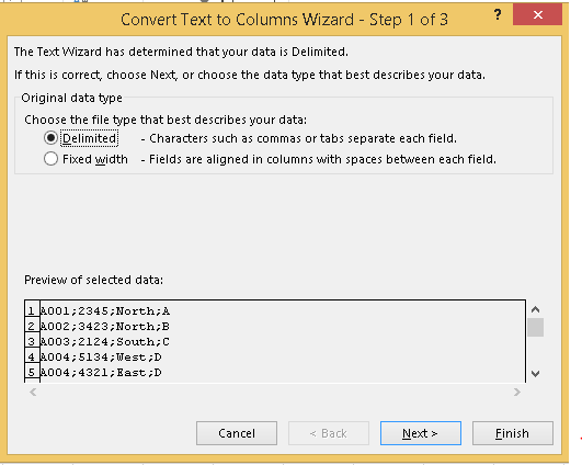
 Above, we have two options "Delimited" and "Fixed width". I have selected delimited because the values are separated by a delimiter (;). If we were interested in dividing the data based on width, as the first four characters in the first column, of the 5 to the 10th character in the second column, then we would choose Fixed width.
 - Click Next -> Check the checkbox to “Semicolon”, then Next and finish.

 Above, we have two options "Delimited" and "Fixed width". I have selected delimited because the values are separated by a delimiter (;). If we were interested in dividing the data based on width, as the first four characters in the first column, of the 5 to the 10th character in the second column, then we would choose Fixed width.
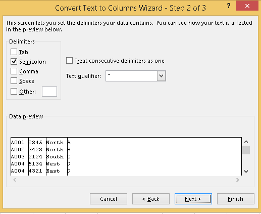
Essential keyboard shortcuts
Keyboard shortcuts are the best way to navigate cells or enter formulas faster. Then, we list our favorites.
- Ctrl +[Down|Up Arrow]: Moves to the top or bottom cell of the current column and the combination of Ctrl with Left | Right arrow , moves to the left or rightmost cell in the current row
- Ctrl + Shift + Up arrow / down: Select all cells above or below the current cell
- Ctrl + Start: Navigate to cell A1
- Ctrl + End: Navigate to the last cell containing data
- Alt + F1: Create a chart based on the selected dataset.
- Ctrl + Shift + L: Activates the automatic filter to the data table
- Alt + Down arrow: To open the auto filter drop-down menu
- Alt + D + S: To sort the data set
- Ctrl + O: Open a new book
- Ctrl + N: Create a new workbook
- F4: Select the range and press the F4 key, will change the reference to absolute, mixed and relative.
Note: this is not an exhaustive list. Feel free to share your favorite keyboard shortcuts in Excel in the comment section below.. Literally, I do the 80% Excel tasks using shortcuts.
Final notes
Excel is arguably one of the best tools ever created and has remained the gold standard for almost every business around the world.. But whether you are a newbie or a power user, there is always something to learn. Or do you think you've seen it all and done it all? Let us know what we missed in the comments..
Do you want to start in the field of data? We have selected the perfect multi-course program for you!! Review the Certified Business Analysis Program and launch your career!


