Target
- Boosting is a joint learning technique in which each model tries to correct the errors of the previous model.
- Aprenda sobre el algoritmo de aumento de gradientGradient is a term used in various fields, such as mathematics and computer science, to describe a continuous variation of values. In mathematics, refers to the rate of change of a function, while in graphic design, Applies to color transition. This concept is essential to understand phenomena such as optimization in algorithms and visual representation of data, allowing a better interpretation and analysis in... y las matemáticas detrás de él.
Introduction
In this article, we are going to discuss an algorithm that works in the impulse technique, the gradient increase algorithm. It is better known as Gradient Boosting Machine or GBM.
Note: If you are more interested in learning concepts in an audiovisual format, we have this full article explained in the video below. If that is not the case, you can keep reading.
The models in Gradient Boosting Machine are being built sequentially and each of these later models tries to reduce the error of the previous model. But the question is how does each model reduce the error of the previous model? It is done by building the new model on errors or residuals of the previous predictions.
This is done to determine if there are any patterns in the error that the previous model ignores. Let's understand this with an example.
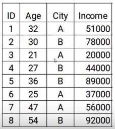
Here we have the data with two characteristics: age and city, and the variableIn statistics and mathematics, a "variable" is a symbol that represents a value that can change or vary. There are different types of variables, and qualitative, that describe non-numerical characteristics, and quantitative, representing numerical quantities. Variables are fundamental in experiments and studies, since they allow the analysis of relationships and patterns between different elements, facilitating the understanding of complex phenomena.... objetivo es el ingreso. Then, according to the city and the age of the person, we have to predict income. Note that throughout the process of increasing gradient, we will update the following: the objective of the model, the residual of the model and the prediction.
Steps to build the gradient augmentation machine model
To simplify the understanding of the gradient augmentation machine, we have divided the process into five simple steps.
Paso 1
The first step is to build a model and make predictions on the given data.. Let's go back to our data, for the first model, the objective will be the Income value given in the data. Then, I have set the target as original Income values.
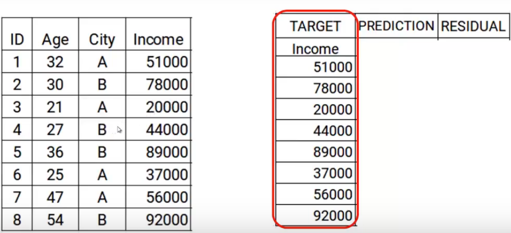
Now we will build the model using the age and city characteristics with the target income. This trained model will be able to generate a set of predictions. Which are assumed as follows.
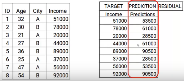
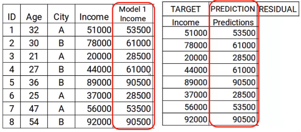
Now I will store these predictions with my data. This is where I complete the first step.
Paso 2
The next step is to use these predictions to get the error, to be used later as a target. At the moment we have the values of Real income and the predictions of the model1. Using these columns, we will calculate the error simply by subtracting the actual revenue and the revenue predictions. A is shown below.
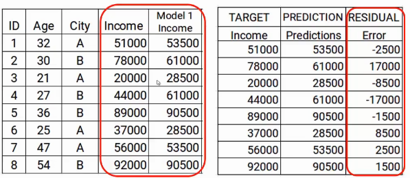
As we mentioned earlier, successive models focus on error. Then, mistakes here will be our new goal. That covers step two.
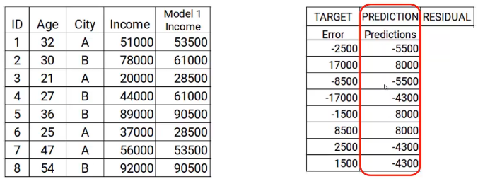
Paso 3
In the next step, we will create a model on these errors and make the predictions. Here the idea is to determine if there are any hidden patterns in the error.
Then, using the error as a target and the original characteristics Age and City, we will generate new predictions. Note that the predictions, in this case, will be the error values, not expected revenue values, since our objective is the error. Let's say the model gives the following predictions
Paso 4
Now we have to update the predictions of model1. We will add the prediction from the previous step and add it to the prediction of model1 and call it Model2 Income.
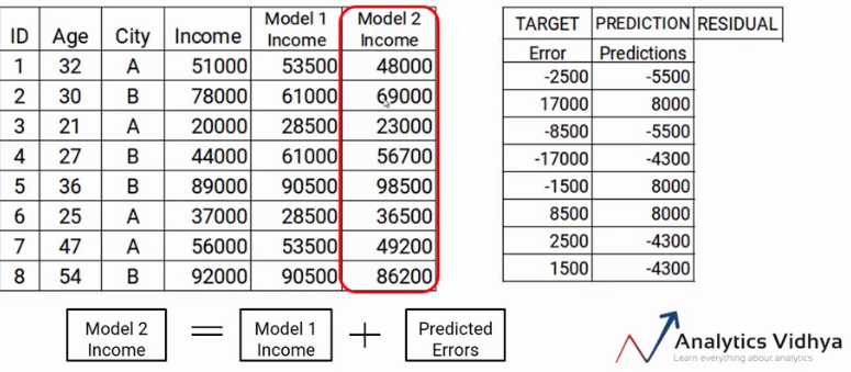
As you can see, my new predictions are closer to the true values of my income.
Finally, we will repeat the steps 2 a 4, which means that we will be calculating new errors and setting this new error as a target. We will repeat this process until the error is zero or we have reached the stop criterion, that says the number of models we want to build. That is the step-by-step process of building a gradient increase model..
In a nutshell, we build our first model that has characteristics x and objective y, Let's call this model H0 which is a function of x and y. Then we build the next model on the errors of the last model and a third model on the errors of the previous model and so on. Until we build n models.
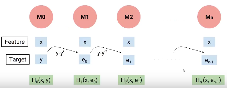
Each successive model works on the errors of all previous models to try to identify any patterns in the error.. effectively, I can say that each of these models are individual functions that have the independent variable x as characteristic and the objective is the error of the previous combined model.
Then, to determine the final equation of our model, we build our first H0 model, which gave me some predictions and generated some errors. Let's call this combined result F0 (X).
Now we create our second model and add new predicted errors to F0 (X), this new function will be F1 (X). Similarly, we will build the following model and so on, until we have n models as shown below.
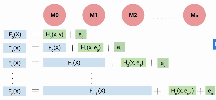
Then, in every step, we try to model the errors, which helps us to reduce the overall error. Ideally, we want this' in’ be zero. As you can see, each model here is trying to increase the performance of the model, Thus, we use the term impulse.
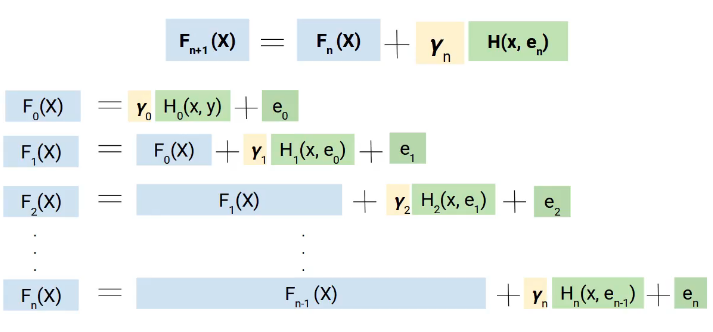
But why do we use the term gradient, here is the trick. Instead of directly adding these models, we add them with weight or coefficient, and the correct value of this coefficient is decided using the gradient increase technique.
Therefore, a more generalized form of our equation will be as follows.
The math behind the Gradient Boosting Machine
Hope now you have a broad idea of how gradient augmentation works. From now on, we will focus on how the value of Yn is calculated.
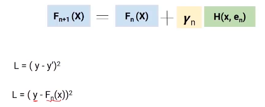
We will use the gradient descent technique to obtain the values of these gamma coefficients (Y), de manera que minimicemos la Loss functionThe loss function is a fundamental tool in machine learning that quantifies the discrepancy between model predictions and actual values. Its goal is to guide the training process by minimizing this difference, thus allowing the model to learn more effectively. There are different types of loss functions, such as mean square error and cross-entropy, each one suitable for different tasks and.... Now let's dive into this equation and understand the role of the loss function and gamma.
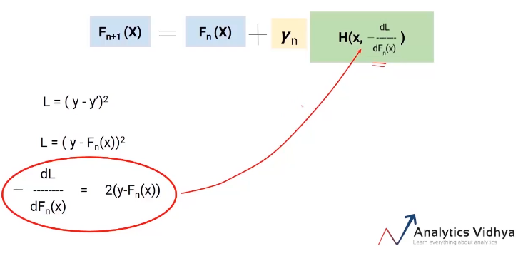
Here, the loss function we are using is (y-y ') 2. y is the real value and y 'is the final value predicted by the last model. Then, we can replace y 'with Fn (X) which represents the actual target minus the updated predictions from all the models we have built so far.
Partial differentiation
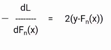
I think you are familiar with the gradient descent process, since we are going to use the same concept. We will differentiate the equation of L with respect to Fn (X), you will get the following equation, which is also known as pseudo residual. What is the negative gradient of the loss function.
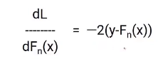
To simplify this, we will multiply both sides by -1. The result will be something like this.
Now, we know that the error in our equation for Fn + 1 (X) is the actual value minus the updated predictions of all models. Therefore, we can replace the en in our final equation with these pseudo residuals as shown in the image below.
So this is our final equation. The best part of this algorithm is that it gives you the freedom to decide the loss function. The only condition is that the loss function is differentiable. To facilitate understanding, we use a very simple loss function (y-y ') 2 but you can change it to hinge loss or logit loss or whatever.
The goal is to minimize total loss. Let's see what the total loss would be here, will be the loss to model n plus the loss of the current model we are building. Here is the equation.
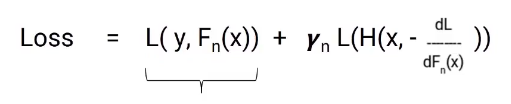
In this equation, the first part is fixed, but the second part is the loss of the model we are currently working on. The loss of this model still cannot be changed, but we can change the value of gamma. Now we have to select the gamma value so that the total loss is minimized and this value is selected by the gradient descent process.
Then, the idea is to reduce the overall loss by deciding the optimal gamma value for each model we build.
Gradient augmentation decision tree
I speak of a special case of gradient increase, namely, gradient magnification decision tree (GBDT). Here, each model would be a tree and the gamma value will be decided at each leaf level, not at the general level of the model. Then, as shown in the following picture, each leaf would have a gamma value.
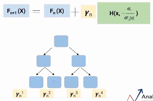
This is how Gradient Boosting Decision Tree works.
Final notes
Boosting is a type of joint learning. It is a sequential process where each model tries to correct the errors of the previous model. This means that each successive model depends on its predecessors.. In this article, we saw the gradient augmentation algorithm and the math behind it.
How we have a clear idea of the algorithm, try to build the models and get some hands-on experience with it.
If you are looking to start your data science journey and want all topics under one roof, your search stops here. Take a look at DataPeaker's certified AI and ML BlackBelt Plus Program
If you have any question, let me know in the comment section!
If you have any question, let me know in the comments below.


