
This post was made public as part of the Data Science Blogathon
Introduction
Python is an easy-to-learn programming language, making it the preferred choice for data science beginners, data analysis and machine learning. It also has a large online student community and excellent data-centric libraries..
With so much data that is generated, it is essential that the data we use for data science applications such as machine learning and predictive modeling is clean. But, What do we understand by clean data? And what messes up the data in the first place?
Dirty data just means bad data. Duplication of records, Incomplete or outdated data and incorrect analysis can mess up the data. This data must be cleaned. Data cleansing (or data cleaning) refers to the procedure of “clean up” this dirty data, identifying errors in the data and then rectifying them.
Data cleansing is an important step in a machine learning project, and we'll cover some basic data cleansing techniques (and Python) in this post.
Data cleaning in Python
We will learn more about data cleansing in Python with the help of a sample data set. We will use the Russian housing data set and Kaggle.
We will start by importing the must-have libraries.
# import libraries
import pandas as pd
import numpy as np
import seaborn as sns
import matplotlib.pyplot as plt
%matplotlib inline
Download the data and then read it in a Pandas DataFrame using the read_csv function () and specifying the file path. Subsequently, use shape attribute to check number of rows and columns in dataset. The code for this is as follows:
df = pd.read_csv('housing_data.csv')
df.shape
The data set has 30 471 rows and 292 columns.
Now we will separate the numeric columns from the categorical columns.
# select numerical columns
df_numeric = df.select_dtypes(include=[np.number])
numeric_cols = df_numeric.columns.values
# select non-numeric columns
df_non_numeric = df.select_dtypes(exclude=[np.number])
non_numeric_cols = df_non_numeric.columns.values
Now we are done with the preliminary steps. Now we can move on to cleaning the data. We will start by identifying columns that contain missing values and try to correct them.
Missing values
We will start by calculating the percentage of missing values in each column and then storing this information in a DataFrame.
# % of values missing in each column
values_list = list()
cols_list = list()
for col in df.columns:
    pct_missing = np.mean(df[col].isnull())*100
    cols_list.append(col)
    values_list.append(pct_missing)
pct_missing_df = pd.DataFrame()
pct_missing_df['col'] = cols_list
pct_missing_df['pct_missing'] = values_list
The DataFrame pct_missing_df now contains the percentage of missing values in each column along with the column names.
We can also create an image from this information for a better understanding using the following code:
pct_missing_df.loc[pct_missing_df.pct_missing > 0].plot(kind='bar', figsize=(12,8))
plt.show()
The result after executing the above line of code should look like this:
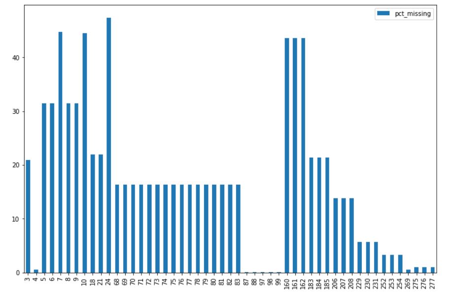
It is clear that some columns are missing very few values, while other columns are missing a substantial percentage of values. Now we will fix these missing values.
There are several ways we can correct these missing values. Some of them are”
Fall observations
One way could be to discard those observations that contain some null value for any of the columns. This will work when the percentage of missing values in each column is much lower. We will eliminate the observations that contain nulls in those columns that have less than 0,5% null. These columns would be metro_min_walk, metro_km_walk, railroad_station_walk_km, railroad_station_walk_min e ID_railroad_station_walk.
less_missing_values_cols_list = list(pct_missing_df.loc[(pct_missing_df.pct_missing < 0.5) & (pct_missing_df.pct_missing > 0), 'col'].values)
df.dropna(subset=less_missing_values_cols_list, inplace=True)
This will reduce the number of records in our dataset to 30,446 records.
Delete columns (functions)
Another way to address missing values in a dataset would be to delete those columns or features that have a significant percentage of missing values.. These columns do not contain much information and can be completely erased from the dataset. In our case, let's eliminate all those columns that are missing more than 40% of values. These columns would be build_year, state, hospital_beds_raion, cafe_sum_500_min_price_avg, cafe_sum_500_max_price_avg y cafe_avg_price_500.
# dropping columns with more than 40% null values
_40_pct_missing_cols_list = list(pct_missing_df.loc[pct_missing_df.pct_missing > 40, 'col'].values)
df.drop(columns=_40_pct_missing_cols_list, inplace=True)
The number of features in our dataset is now 286.
Impute missing values
Data is still missing in our dataset. Now we will impute the missing values in each numeric column with the median value of that column.
df_numeric = df.select_dtypes(include=[np.number])
numeric_cols = df_numeric.columns.values
for col in numeric_cols:
    missing = df[col].isnull()
    num_missing = np.sum(missing)
    if num_missing > 0:  # impute values only for columns that have missing values
        med = df[col].median() #impute with the median
        df[col] = df[col].fillna(with)
Missing values in numeric columns are now fixed. In the case of categorical columns, we will replace the missing values with the fashion values of that column.
df_non_numeric = df.select_dtypes(exclude=[np.number])
non_numeric_cols = df_non_numeric.columns.values
for col in non_numeric_cols:
    missing = df[col].isnull()
    num_missing = np.sum(missing)
    if num_missing > 0:  # impute values only for columns that have missing values
        mod = df[col].describe()['top'] # impute with the most frequently occuring value
        df[col] = df[col].fillna(mod)
All missing values in our dataset have already been dealt with. We can verify this by running the following code:
df.isnull().sum().sum()
If the output is zero, means now there are no missing values left in our dataset.
Furthermore we can replace the missing values with a particular value (What -9999 the 'missing') which will indicate the fact that the data was missing in this place. This can be a substitute for the imputation of lost value.
Atypical values
An outlier is an unusual observation that deviates from most of the data. Outliers can significantly affect the performance of a machine learning model. Therefore, identifying outliers and addressing them is essential.
Let's take the column ‘life_sq’ as an example. We will first use the describe method () to look at the descriptive statistics and see if we can collect information from it.
df.life_sq.describe()
The output will look like this:
count    30446.000000
mean        33.482658
std         46.538609
min          0.000000
25%         22.000000
50%         30.000000
75%         38.000000
max       7478.000000
Name: life_sq, dtype: float64
Of departure, it is clear that something is not correct. The maximum value appears to be abnormally large compared to the mean and median values. Let's make a box plot of this data to get a better idea.
df.life_sq.plot(kind='box', figsize=(12, 8))
plt.show()
The output will look like this:
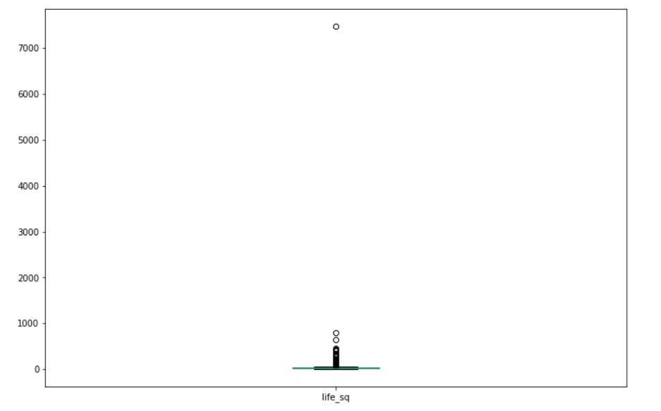
From the box plot it is clear that the observation for the maximum value (7478) is an outlier in this data. Descriptive statistics, the box plotsBox Diagrams, Also known as box and whisker diagrams, are statistical tools that represent the distribution of a dataset. These diagrams show the median, quartiles and outliers, allowing data variability and symmetry to be visualized. They are useful in comparison between different groups and in exploratory analysis, making it easier to identify trends and patterns in the data.... y los diagramas de dispersión nos ayudan a identificar valores atípicos en los datos.
We can deal with outliers like we did with missing values. We can delete the observations that we think are outliers, or we can replace outliers with suitable values, or we can do some kind of transformation on the data (as logarithm or exponential). In our case, let's delete the record where the value of ‘life_sq’ it is 7478.
# removing the outlier value in life_sq column
df = df.loc[df.life_sq < 7478]
Duplicate records
Sometimes, data can contain duplicate values. It is essential to clear duplicate records from your dataset before proceeding with any machine learning project. In our data, since the ID column is a unique identifier, we will eliminate duplicate records considering all but the ID column.
# dropping duplicates by considering all columns other than ID
cols_other_than_id = list(df.columns)[1:]
df.drop_duplicates(subset=cols_other_than_id, inplace=True)
This will help us to erase duplicate records. When using the shape method, you can verify that the duplicate records have truly been removed. The number of observations is now 30,434.
Fixing the data type
Often, in the data set, values are not stored in correct data type. This can create a roadblock in later stages and we may not get the desired result or get errors during execution.. A common data type error is dates. Dates are often parsed as objects in Python. There is a separate data type for dates in Pandas, called DateTime.
We will first check the data type of the timestamp column in our data.
df.timestamp.dtype
This returns the data type 'object'. Now we know that the timestamp is not stored correctly. To fix this problem, convert timestamp column to DateTime format.
# converting timestamp to datetime format
df['timestamp'] = pd.to_datetime(df.timestamp, format="%Y-%m-%d")
Now we have the timestamp in the correct format. Similarly, there can be columns where integers are stored as objects. It is essential to identify these characteristics and correct the data type before proceeding with machine learning.. Lucky for us, we don't have any such problems in our dataset.
EndNote
In this post, We discussed some basic ways that we can clean data in Python before starting our machine learning project. We need to identify and erase the missing values, identify and address outliers, clear duplicate records and correct the data type of all columns in our dataset before continuing with our AA task.
The author of this post is Vishesh Arora. You can connect with me at LinkedIn.
The media shown in this post about sign language accreditation is not the property of DataPeaker and is used at the author's discretion.





