OpenCV image processing | Image processing with OpenCV

Introduction

Hello readers!

OpenCV – Open source computer vision. It is one of the most used tools for image processing and artificial vision tasks. Used in various applications such as face detection, video capture, tracking moving objects, revelation of objects, nowadays in Covid applications such as mask detection, social distancing and many more. If you want to know more about OpenCV, check this Link.

📌If you want to learn more about Python libraries for image processing, check this link.

📌If you want to learn how to process images using NumPy, 😋check this link.

📌For more articles😉, Click here

In this blog, I will cover OpenCV in great detail covering some of the most important tasks in image processing through practical implementation. So let's get started !! ⌛

Image Source

Table of Contents

• Edge detection and image gradients
• Dilatation, opening, closure and erosion
• Perspective transformation
• Pyramids of images
• Trim
• climbed, interpolations and resizing
• Thresholding, adaptive thresholding and binarization
• Sharp
• Blot
• contours
• Line detection using hard lines
• Find corners
• Counting circles and ellipses

Image Source

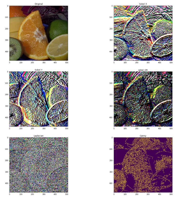
Edge detection and image gradients

It is one of the most fundamental and important techniques in image processing. Check the code below for a full implementation. For more information, see this Link.

image = cv2.imread('fruit.jpg')
image = cv2.cvtColor(image, cv2.COLOR_BGR2RGB)
hgt, wdt,_ = image.shape
# Sobel Edges
x_sobel = cv2.Sobel(image, cv2.CV_64F, 0, 1, ksize=5)
y_sobel = cv2.Sobel(image, cv2.CV_64F, 1, 0, ksize=5)
plt.figure(figsize=(20, 20))
plt.subplot(3, 2, 1)
plt.title("Original")
plt.imshow(image)
plt.subplot(3, 2, 2)
plt.title("Sobel X")
plt.imshow(x_sobel)
plt.subplot(3, 2, 3)
plt.title("Sobel Y")
plt.imshow(y_sobel)
sobel_or = cv2.bitwise_or(x_sobel, y_sobel)
plt.subplot(3, 2, 4)
plt.imshow(sobel_or)
laplacian = cv2.Laplacian(image, cv2.CV_64F)
plt.subplot(3, 2, 5)
plt.title("Laplacian")
plt.imshow(laplacian)
## There are two values: threshold1 and threshold2.
## Those gradients that are greater than threshold2 => considered as an edge
## Those gradients that are below threshold1 => considered not to be an edge.
## Those gradients Values that are in between threshold1 and threshold2 => either classified as edges or non-edges
# The first threshold gradient
canny = cv2.Canny(image, 50, 120)
plt.subplot(3, 2, 6)
plt.imshow(canny)

Dilatation, opening, closure and erosion

These are two fundamental image processing operations. They are used to eliminate noise, find a hole of intensity or a bump in an image and many more. See the following code for a practical implementation. For more information, see this Link.

image = cv2.imread('LinuxLogo.jpg')
image = cv2.cvtColor(image, cv2.COLOR_BGR2RGB)
plt.figure(figsize=(20, 20))
plt.subplot(3, 2, 1)
plt.title("Original")
plt.imshow(image)

kernel = np.ones((5,5), e.g. uint8)

erosion = cv2.erode(image, kernel, iterations = 1)
plt.subplot(3, 2, 2)
plt.title("Erosion")
plt.imshow(erosion)
dilation = cv2.dilate(image, kernel, iterations = 1)
plt.subplot(3, 2, 3)
plt.title("Dilation")
plt.imshow(dilation)

opening = cv2.morphologyEx(image, cv2.MORPH_OPEN, kernel)
plt.subplot(3, 2, 4)
plt.title("Opening")
plt.imshow(opening)

closing = cv2.morphologyEx(image, cv2.MORPH_CLOSE, kernel)
plt.subplot(3, 2, 5)
plt.title("Closing")
plt.imshow(closing)

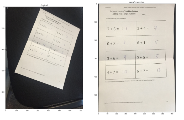
Perspective transformation

To get better information about an image, we can change the perspective of a video or an image. In this transformation, we need to provide the points in an image from where we want to take information by changing the perspective. En OpenCV, we use two functions for perspective transformation getPerspectiveTransform () and later warpPerspective (). Check the code below for a full implementation. For more information, see this Link.

image = cv2.imread('scan.jpg')
image = cv2.cvtColor(image, cv2.COLOR_BGR2RGB)
plt.figure(figsize=(20, 20))
plt.subplot(1, 2, 1)
plt.title("Original")
plt.imshow(image)
points_A = np.float32([[320,15], [700,215], [85,610], [530,780]])
points_B = np.float32([[0,0], [420,0], [0,594], [420,594]])
M = cv2.getPerspectiveTransform(points_A, points_B)
warped = cv2.warpPerspective(image, M, (420,594))
plt.subplot(1, 2, 2)
plt.title("warpPerspective")
plt.imshow(warped)

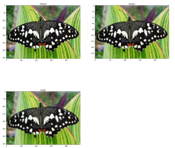
Pyramids of images

It is a very useful technique when we need to scale in the detection of objects. OpenCV uses two common types of image pyramids Gaussiano y Laplaciano pyramid. Use the live () Y pyrDown () function in OpenCV to reduce or enlarge an image. See the following code for a practical implementation. For more information, see this Link.

image = cv2.imread('butterfly.jpg')
image = cv2.cvtColor(image, cv2.COLOR_BGR2RGB)
plt.figure(figsize=(20, 20))
plt.subplot(2, 2, 1)
plt.title("Original")
plt.imshow(image)
smaller = cv2.pyrDown(image)
larger = cv2.pyrUp(smaller)
plt.subplot(2, 2, 2)
plt.title("Smaller")
plt.imshow(smaller)
plt.subplot(2, 2, 3)
plt.title("Larger")
plt.imshow(larger)

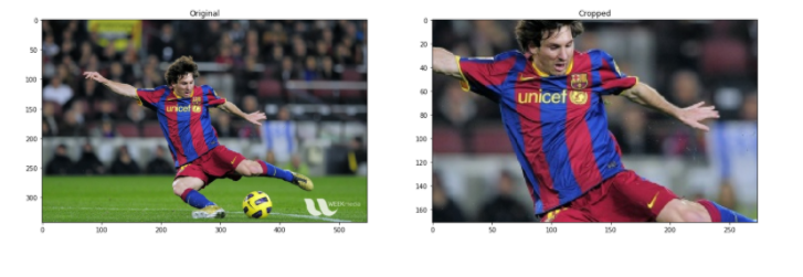
Trim

It is one of the most important and fundamental techniques in image processing, cropping is used to obtain a particular part of an image. To crop an image. You only need the coordinates of an image according to your area of ​​interest. For a complete analysis, see the following code in OpenCV.

image = cv2.imread('messi.jpg')
image = cv2.cvtColor(image, cv2.COLOR_BGR2RGB)
plt.figure(
Aigsize=(20, 20))
plt.subplot(2, 2, 1)
plt.title("Original")
plt.imshow(image)
hgt, wdt = image.shape[:2]
start_row, start_col = int(hgt * .25), int(wdt * .25)
end_row, end_col = int(height * .75), int(width * .75)
cropped = image[start_row:end_row , start_col:end_col]
plt.subplot(2, 2, 2)
plt.imshow(cropped)

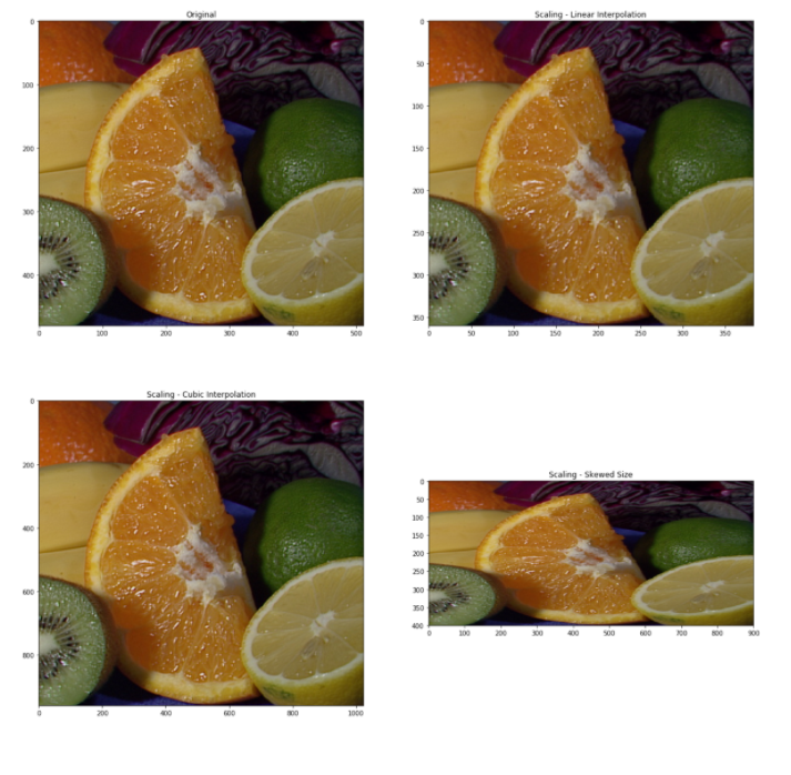
climbed, interpolations and resizing

Resizing it is one of the simplest tasks in OpenCV. Provides a resize () Function Taking parametersThe "parameters" are variables or criteria that are used to define, measure or evaluate a phenomenon or system. In various fields such as statistics, Computer Science and Scientific Research, Parameters are critical to establishing norms and standards that guide data analysis and interpretation. Their proper selection and handling are crucial to obtain accurate and relevant results in any study or project.... as image, output size image, interpolation, x scale and y scale. Check the code below for a full implementation.

image = cv2.imread('/kaggle/input/opencv-samples-images/data/fruits.jpg')
image = cv2.cvtColor(image, cv2.COLOR_BGR2RGB)
plt.figure(figsize=(20, 20))
plt.subplot(2, 2, 1)
plt.title("Original")
plt.imshow(image)
image_scaled = cv2.resize(image, None, fx=0.75, fy=0.75)
plt.subplot(2, 2, 2)
plt.title("Scaling - Linear Interpolation")
plt.imshow(image_scaled)
img_scaled = cv2.resize(image, None, fx=2, fy=2, interpolation = cv2.INTER_CUBIC)
plt.subplot(2, 2, 3)
plt.title("Scaling - Cubic Interpolation")
plt.imshow(img_scaled)
img_scaled = cv2.resize(image, (900, 400), interpolation = cv2.INTER_AREA)
plt.subplot(2, 2, 4)
plt.title("Scaling - Skewed Size")
plt.imshow(img_scaled)

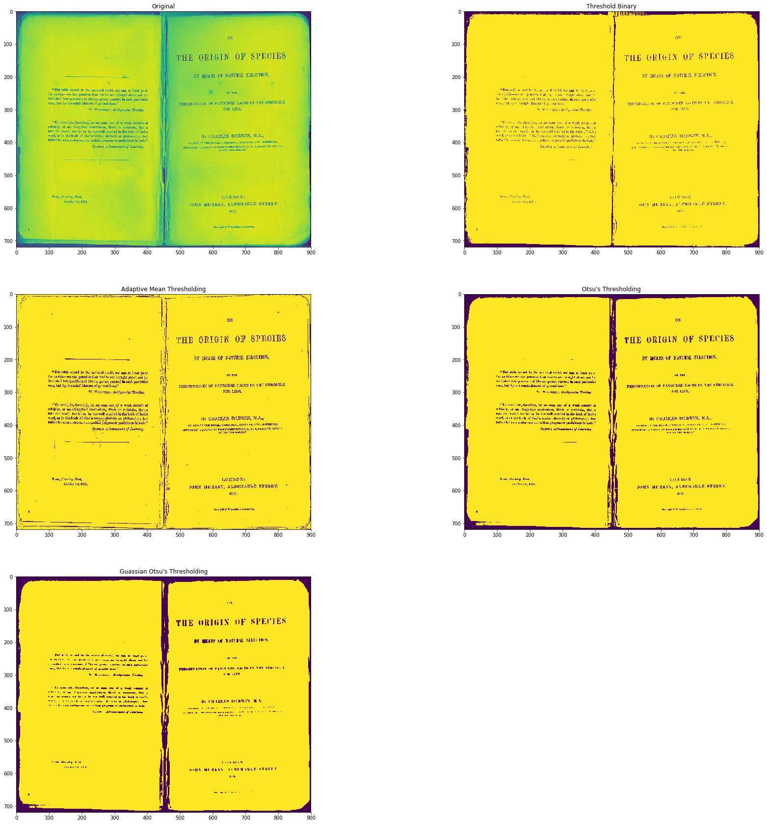
Thresholding, adaptive thresholding and binarization

Check the code below for a full implementation. For more information, see this Link.

# Load our new image
image = cv2.imread('Origin_of_Species.jpg', 0)
plt.figure(figsize=(30, 30))
plt.subplot(3, 2, 1)
plt.title("Original")
plt.imshow(image)
right,thresh1 = cv2.threshold(image, 127, 255, cv2.THRESH_BINARY)
plt.subplot(3, 2, 2)
plt.title("Threshold Binary")
plt.imshow(thresh1)
image = cv2.GaussianBlur(image, (3, 3), 0)
thresh = cv2.adaptiveThreshold(image, 255, cv2.ADAPTIVE_THRESH_MEAN_C, cv2.THRESH_BINARY, 3, 5) 
plt.subplot(3, 2, 3)
plt.title("Adaptive Mean Thresholding")
plt.imshow(thresh)
_, th2 = cv2.threshold(image, 0, 255, cv2.THRESH_BINARY + cv2.THRESH_OTSU)
plt.subplot(3, 2, 4)
plt.title("Otsu's Thresholding")
plt.imshow(th2)
plt.subplot(3, 2, 5)
blur = cv2.GaussianBlur(image, (5,5), 0)
_, th3 = cv2.threshold(blur, 0, 255, cv2.THRESH_BINARY + cv2.THRESH_OTSU)
plt.title("Guassian Otsu's Thresholding")
plt.imshow(th3)
plt.show()

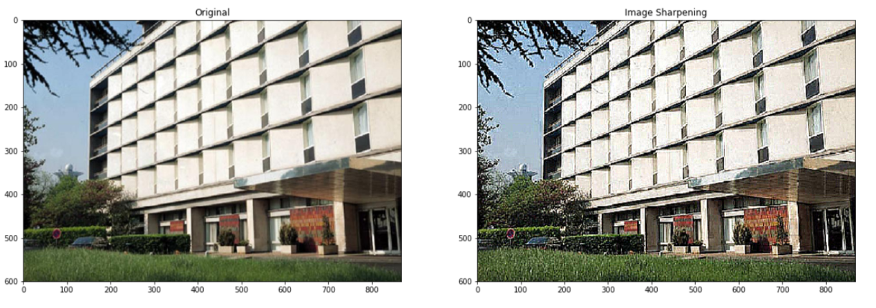
Sharp

Check the following code to focus an image using OpenCV. For more information, see this Link

image = cv2.imread('building.jpg')
image = cv2.cvtColor(image, cv2.COLOR_BGR2RGB)
plt.figure(figsize=(20, 20))
plt.subplot(1, 2, 1)
plt.title("Original")
plt.imshow(image)
kernel_sharpening = np.array([[-1,-1,-1], 
                              [-1,9,-1], 
                              [-1,-1,-1]])
sharpened = cv2.filter2D(image, -1, kernel_sharpening)
plt.subplot(1, 2, 2)
plt.title("Image Sharpening")
plt.imshow(sharpened)
plt.show()

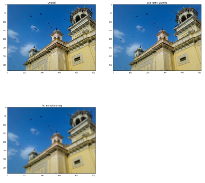
Blot

Check the following code to blur an image using OpenCV. For more information, see this Link

image = cv2.imread('home.jpg')
image = cv2.cvtColor(image, cv2.COLOR_BGR2RGB)
plt.figure(figsize=(20, 20))
plt.subplot(2, 2, 1)
plt.title("Original")
plt.imshow(image)
kernel_3x3 = np.ones((3, 3), e.g. float32) / 9
blurred = cv2.filter2D(image, -1, kernel_3x3)
plt.subplot(2, 2, 2)
plt.title("3x3 Kernel Blurring")
plt.imshow(blurred)
kernel_7x7 = np.ones((7, 7), e.g. float32) / 49
blurred2 = cv2.filter2D(image, -1, kernel_7x7)
plt.subplot(2, 2, 3)
plt.title("7x7 Kernel Blurring")
plt.imshow(blurred2)

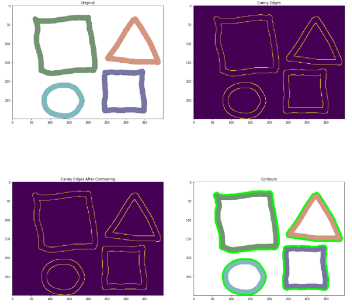
contours

# Load the data
image = cv2.imread('pic.png')
image = cv2.cvtColor(image, cv2.COLOR_BGR2RGB)
plt.figure(figsize=(20, 20))
plt.subplot(2, 2, 1)
plt.title("Original")
plt.imshow(image)
# Grayscale
gray = cv2.cvtColor(image,cv2.COLOR_BGR2GRAY)
# Canny edges
edged = cv2.Canny(gray, 30, 200)
plt.subplot(2, 2, 2)
plt.title("Canny Edges")
plt.imshow(edged)
# Finding Contours
contour, here = cv2.findContours(edged, cv2.RETR_EXTERNAL, cv2.CHAIN_APPROX_NONE)
plt.subplot(2, 2, 3)
plt.imshow(edged)
print("Count of Contours  = " + str(len(contour)))
# All contours
cv2.drawContours(image, contours, -1, (0,255,0), 3)
plt.subplot(2, 2, 4)
plt.title("Contours")
plt.imshow(image)

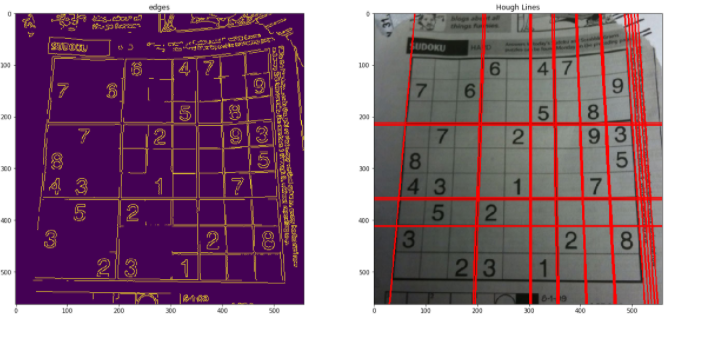
Line detection using hard lines

Lines can be detected in an image using Hough lines. OpenCV provides a HouhLines function in which the threshold value should pass. The threshold is the minimum vote for a line to be considered. For a detailed description, see the following code for a full implementation. For line detection using Hough lines in OpenCV. For more information, see this Link.

# Load the image
image = cv2.imread('sudoku.png')
image = cv2.cvtColor(image, cv2.COLOR_BGR2RGB)
plt.figure(figsize=(20, 20))
# Grayscale 
gray = cv2.cvtColor(image, cv2.COLOR_BGR2GRAY)
# Canny Edges
edges = cv2.Canny(gray, 100, 170, apertureSize = 3)
plt.subplot(2, 2, 1)
plt.title("edges")
plt.imshow(edges)
# Run HoughLines Fucntion 
lines = cv2.HoughLines(edges, 1, np.pi/180, 200)
# Run for loop through each line
for line in lines:
    rho, theta = line[0]
    a = np.cos(theta)
    b = np.sin(theta)
    x0 = a * rho
    y0 = b * rho
    x_1 = int(x0 + 1000 * (-b))
    y_1 = int(y0 + 1000 * (a))
    x_2 = int(x0 - 1000 * (-b))
    y_2 = int(y0 - 1000 * (a))
    cv2.line(image, (x_1, y_1), (x_2, y_2), (255, 0, 0), 2)
# Show Final output
plt.subplot(2, 2, 2)
plt.imshow(image)

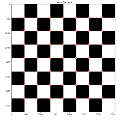
Find corners

To find the corners of an image, use el cornerHarris function from OpenCV. For a detailed overview, see the code below for a full implementation to find corners using OpenCV. For more information, see this Link.

# Load image 
image = cv2.imread('chessboard.png')
# Grayscaling
image = cv2.cvtColor(image, cv2.COLOR_BGR2RGB)
plt.figure(figsize=(10, 10))
gray = cv2.cvtColor(image, cv2.COLOR_BGR2GRAY)
# CornerHarris function  want input to be float
gray = np.float32(gray)
h_corners = cv2.cornerHarris(gray, 3, 3, 0.05)
kernel = np.ones((7,7),e.g. uint8)
h_corners = cv2.dilate(harris_corners, kernel, iterations = 10)
image[h_corners > 0.024 * h_corners.max() ] = [256, 128, 128]
plt.subplot(1, 1, 1)
# Final Output
plt.imshow(image)

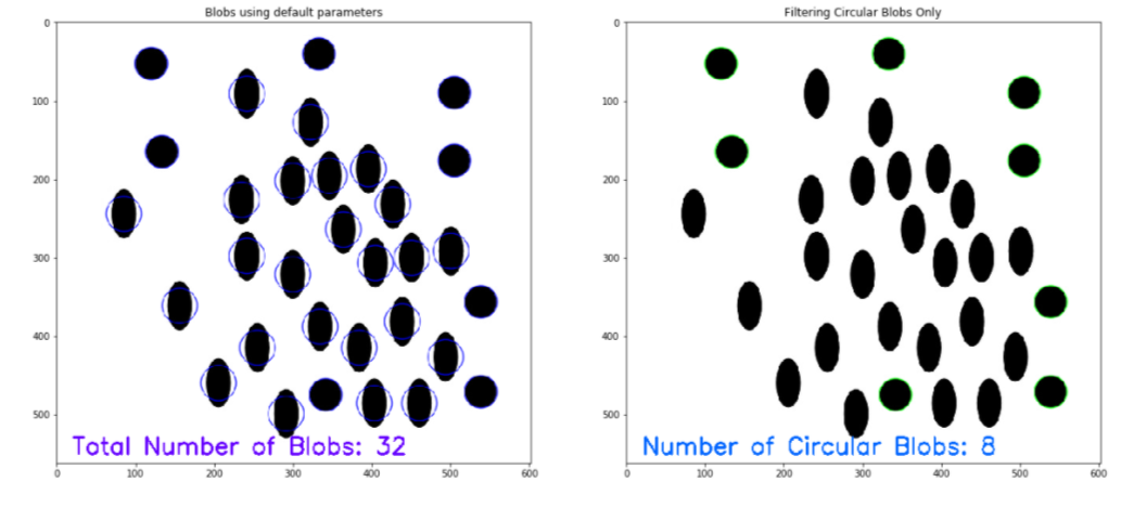
Counting circles and ellipses

To count circles and ellipse in a picture, use el SimpleBlobDetector function from OpenCV. For a detailed overview, see code below for full implementation To Count Circles and Ellipse in an image using OpenCV. For more information, see this Link.

# Load image
image = cv2.imread('blobs.jpg')
image = cv2.cvtColor(image, cv2.COLOR_BGR2RGB)
plt.figure(figsize=(20, 20))
detector = cv2.SimpleBlobDetector_create()
# Detect blobs
points = detector.detect(image)

blank = np.zeros((1,1)) 
blobs = cv2.drawKeypoints(image, points, blank, (0,0,255),
                                      cv2.DRAW_MATCHES_FLAGS_DRAW_RICH_KEYPOINTS)
number_of_blobs = len(keypoints)
text = "Total Blobs: " + str(len(keypoints))
cv2.putText(blobs, text, (20, 550), cv2.FONT_HERSHEY_SIMPLEX, 1, (100, 0, 255), 2)

plt.subplot(2, 2, 1)

plt.imshow(blobs)
# Filtering parameters
# Initialize parameter settiing using cv2.SimpleBlobDetector
params = cv2.SimpleBlobDetector_Params()
# Area filtering parameters
params.filterByArea = True
params.minArea = 100
# Circularity filtering parameters
params.filterByCircularity = True 
params.minCircularity = 0.9
# Convexity filtering parameters
params.filterByConvexity = False
params.minConvexity = 0.2
#  inertia filtering parameters
params.filterByInertia = True
params.minInertiaRatio = 0.01
# detector with the parameters
detector = cv2.SimpleBlobDetector_create(params)
# Detect blobs
keypoints = detector.detect(image)
# Draw blobs on our image as red circles
blank = np.zeros((1,1)) 
blobs = cv2.drawKeypoints(image, keypoints, blank, (0,255,0),
                                      cv2.DRAW_MATCHES_FLAGS_DRAW_RICH_KEYPOINTS)
number_of_blobs = len(keypoints)
text = "No.  Circular Blobs: " + str(len(keypoints))
cv2.putText(blobs, text, (20, 550), cv2.FONT_HERSHEY_SIMPLEX, 1, (0, 100, 255), 2)
# Show blobs
plt.subplot(2, 2, 2)
plt.title("Filtering Circular Blobs Only")
plt.imshow(blobs)

Final notes

Then, in this article, we had a detailed discussion about Image processing using OpenCV. Hope you learn something from this blog and help you in the future. Thanks for reading and your patience. Good luck!

You can check my articles here: Articles

Email identification: [email protected]

Connect with me on LinkedIn: LinkedIn

Media shown in this OpenCV image processing article is not the property of DataPeaker and is used at the author's discretion.

Related