Order statistics | What are order statistics?

The K^th the order statistic for this experiment is k^th smallest value of the set {4, 2, 7, 11, 5}. Then, the 1^{S t} the order statistic is 2 (smallest value), the 2^{North Dakota} the order statistic is 4 (the next smallest), and so on. The 5^th the order statistic is the fifth smallest value (the greatest value), What is it 11. We repeat this process many times, namely, we extract samples from the distribution of each of these iid random variables and find the k^th smallest value for each set of observations. The probability distribution of these values ​​gives the distribution of k^th order statistics.

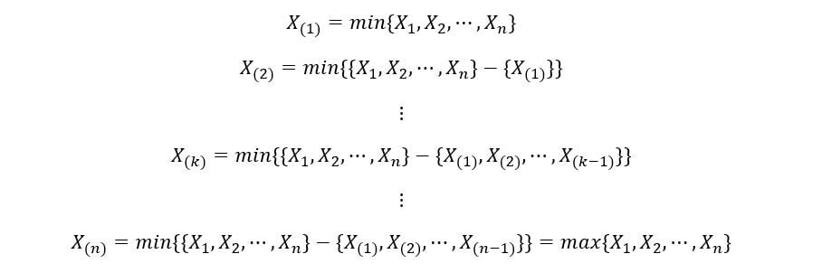
In general, if we order random variables X₁, X₂, …, X_North in ascending order, then the k^th the order statistic is displayed as:

The general notation of the k^th the order statistic is X_(k). Note X_(k) is different from X_k. X_k is the k^th random variable of our set, while X_(k) is the k^th statistical order of our set. X_(k) takes the value of X_k yes X_k is the k^th Random variable when realizations are sorted in ascending order.

The 1^{S t} X-order statistic₍₁₎ is the set of minimum values ​​of the realization of the set of 'n’ random variables. Later^th X-order statistic_(North) is the set of maximum values (nth minimum values) of the realization of the set of 'n’ random variables. They can be expressed as:

Order statistics distribution

Now we will try to find out the distribution of the order statistics. We will first describe the distribution of the n^th order statistics, then he 1^{S t} statistical order and finally the k^th general order statistics.

A) Distribution of n^th Order statistics:

Let the probability density function (PDF) and the cumulative distribution function (CDF) our random variables let f_X(x) y F_X(x) respectively. By definition of CDF,

Since our random variables are identically distributed, have the same PDF f_X(x) y CDF F_X(X). Now we will calculate the CDF of n^th order statistics (F_North(x)) as follows:

Random variables X₁, X₂, …, X_North they are also independent. Therefore, by property of independence,

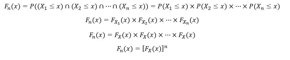
The PDF of the n^th statistical order (f_North(x)) is calculated as follows:

Therefore, the expression for PDF and CDF of n^th The order statistic has been obtained.

B) Distribution of 1^{S t} Order statistics:

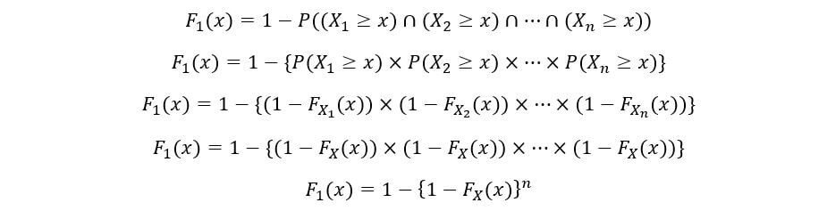
The CDF of a random variable can also be calculated as the one minus the probability that the random variable X takes a value greater than or equal to x. Mathematically,

We will determine the CDF of 1^{S t} order statistics (F₁(x)) as follows:

One more time, using the independence property of random variables,

The PDF of the 1^{S t} statistical order (f₁(x)) is calculated as follows:

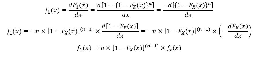
Therefore, the expression for PDF and CDF of 1^{S t} The order statistic has been obtained.

C) Distribution of the k^th Order statistics:

Fork^th order statistics, in general, the following equation describes your CDF (F_k(X)):

The PDF of k^th statistical order (f_k(x)) is expressed as:

To prevent confusions, we will use geometric proofs to understand the equation. As discussed above, the set of random variables has the same PDF (f_X(X)). The graphic below shows a sample PDF with the k^th Order statistic obtained from random sampling:

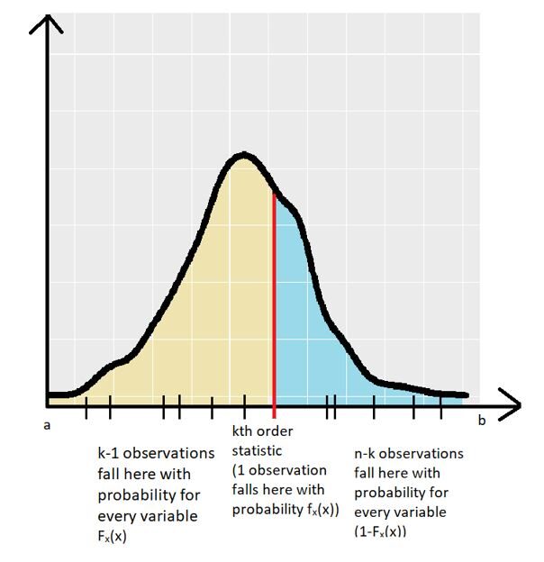
Then, the PDF of the random variables f_X(x) is defined between the interval [a,b]. The k-th order statistic for a random sample is shown with the red line. The other variable realizations (for the random sample) shown by the small black lines on the x-axis.

There are exactly (k – 1) observations of random variables that fall in the yellow region of the graph (the region between & k^th order statistics). The probability that a particular observation falls into this region is given by the CDF of the random variables (F_X(X)). But we are aware that (k – 1) observations fell in the region, what gives us the term (for independence) (F_X(X))^{(k – 1)}.

There are exactly (n – k) observations of random variables that fall in the blue region of the graph (the region between k^th statistical order & b). The probability that a particular observation will fall in this region is given by the 1 – CDF of the random variables (1– F_X(X)). But we are aware that (n – k) observations fell in the region, what gives us the term (for independence) (1-F_X(X))^{(n – k)}.

Finally, exactly 1 observation falls exactly on the k-th order statistic with probability f_X(X). Therefore, the product of 3 terms gives us an idea of ​​the geometric meaning of the equation for PDF of the k-th order statistic. But, Where does the factorial term come from? The above scenario only showed one of the many orderings. There can be many of these combinations. The total number of such combinations is shown below:

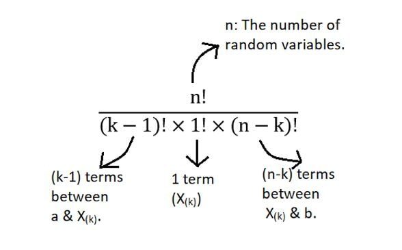
Therefore, the product of all these terms gives us the general distribution of k^th order statistics.

Useful functions of order statistics

Order statistics lead to several useful functions. Among them, notable ones include the sample range and the medianThe median is a statistical measure that represents the central value of a set of ordered data. To calculate it, the data is organized from lowest to highest and the number in the middle is identified. If there are an even number of observations, the two core values are averaged. This indicator is especially useful in asymmetric distributions, since it is not affected by extreme values.... of the sample.

1) Sample range: It is defined as the difference between the largest and smallest value. It is expressed as follows:

2) Sample median: The sample median divides the random sample (realizations of the set of random variables) in two halves, one containing the lowest value samples and the other containing the highest value samples. It's like the middle order statistic / central. It is mathematically defined as:

Order statistics set PDF

A joint probability density function can help us better understand the relationship between two random variables (two-order statistics
in our case). The joint PDF for any statistics of 2 X orders_(a) & X_(B), such that 1 ≤ a ≤ b ≤ n is given by the following equation:

Example

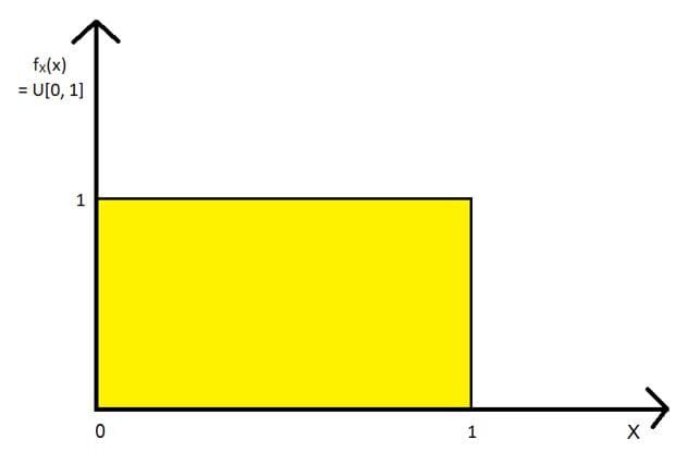
We will use a very simple example to illustrate the distribution of the order statistics: the standard uniform distribution (U[0, 1] distribution). We will take 5 random variables X₁, X₂, X₃, X₄, X₅, everyone has the U[0, 1] distribution. For this set of random variables, we will calculate and plot the 1^{S t}, 3^rd (the sample median) Y 5^th (North^th) order statistics. The following figure"Figure" is a term that is used in various contexts, From art to anatomy. In the artistic field, refers to the representation of human or animal forms in sculptures and paintings. In anatomy, designates the shape and structure of the body. What's more, in mathematics, "figure" it is related to geometric shapes. Its versatility makes it a fundamental concept in multiple disciplines.... shows the U[0, 1] distribution:

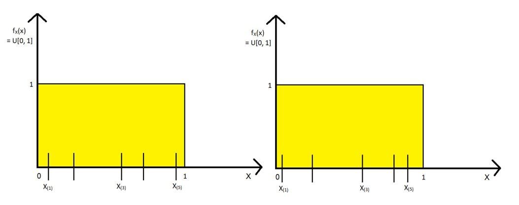
We will draw random samples as follows and find the 1^{S t}, 3^rd & 5^th order statistic for each sample. Below are two of the samples:

The standard uniform distribution PDF and CDF are given as:

We will use this information and calculate X₍₁₎, X₍₃₎ & X₍₅₎ using the formulas we derived. We will take the case only when x is between 0 Y 1 (for other cases, the order statistic is zero since PDF is zero).

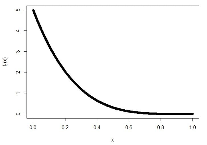
A) To 1^{S t} order statistics:

Plot for f₁(X):

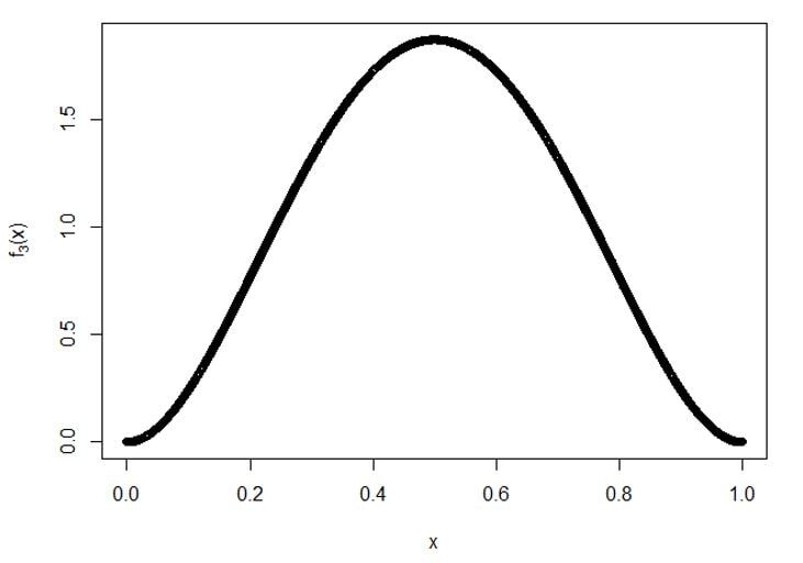
B) To 3^rd order statistics:

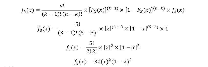
Plot for f₅(X):

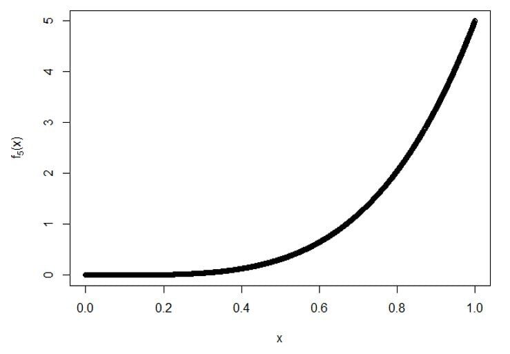
C) To 5^th order statistics:

Plot for f₅(X):

Conclution

Therefore, we have explored the concepts of order statistics in depth. A wide range of physical processes can be modeled through order statistics, exploiting its properties, particularly their distributions.

The media shown in this article is not the property of DataPeaker and is used at the author's discretion.

Related