Introduction
Occasionally, se desarrolla una biblioteca de Python que tiene el potencial de cambiar el panorama en el campo del deep learningDeep learning, A subdiscipline of artificial intelligence, relies on artificial neural networks to analyze and process large volumes of data. This technique allows machines to learn patterns and perform complex tasks, such as speech recognition and computer vision. Its ability to continuously improve as more data is provided to it makes it a key tool in various industries, from health.... PyTorch is one of those libraries.
In the last weeks, I've been dabbling in PyTorch a bit. I was impressed by how easy it is to understand. Among the various deep learning frameworks that I have used to date, PyTorch has been the most flexible and effortless of all.
![]()
In this article, we will explore PyTorch with a more practical approach, covering the basics along with a case study. También compararemos una red neuronalNeural networks are computational models inspired by the functioning of the human brain. They use structures known as artificial neurons to process and learn from data. These networks are fundamental in the field of artificial intelligence, enabling significant advancements in tasks such as image recognition, Natural Language Processing and Time Series Prediction, among others. Their ability to learn complex patterns makes them powerful tools.. construida desde cero tanto en numpy como en PyTorch para ver sus similitudes en la implementación.
Let's move on!
Note: this article assumes you have a basic understanding of deep learning. If you want to catch up on deep learning, read this article first.
What's more, if you want a more detailed explanation of PyTorch from scratch, understand how tensioners work, how you can perform math and matrix operations with PyTorch, I highly recommend that you check out A Beginner's Guide to PyTorch and How It Works From Scratch.
Table of Contents
- An overview of PyTorch
- Dive into the technicalities
- Building a neural network in Numpy vs. PyTorch
- Comparison with other deep learning libraries
- Case study: solving an image recognition problem with PyTorch
If you prefer to address the following concepts in a structured format, You can enroll in this free course at PyTorch and follow them by chapters.
An overview of PyTorch
The creators of PyTorch say they have a philosophy: they want to be imperative. This means that we run our calculation immediately. This fits perfectly into the Python programming methodology, What we don't have to wait for all the code to be written before we know if it works or not. We can easily execute a part of the code and inspect it in real time. For me, as a neural network debugger, This is a blessing!
PyTorch is a Python-based library created to provide flexibility as a deep learning development platform. PyTorch workflow is the closest thing to Python's scientific computing library: numpy.
Now i might ask, Why would we use PyTorch to build deep learning models? I can list three things that could help answer that:
- Easy to use API – It is as simple as Python can be.
- Python support – As mentioned earlier, PyTorch integrates seamlessly with the Python data science stack. It's so similar to numpy that you might not even notice the difference.
- Dynamic calculation graphs – Instead of predefined charts with specific functionalities, PyTorch proporciona un marco para que construyamos gráficos computacionales a measureThe "measure" it is a fundamental concept in various disciplines, which refers to the process of quantifying characteristics or magnitudes of objects, phenomena or situations. In mathematics, Used to determine lengths, Areas and volumes, while in social sciences it can refer to the evaluation of qualitative and quantitative variables. Measurement accuracy is crucial to obtain reliable and valid results in any research or practical application.... que avanzamos, and we even change them during runtime. This is valuable for situations where we don't know how much memory it will take to create a neural network..
Some other advantages of using PyTorch are its multiGPU support, custom data loaders and simplified preprocessors.
Since its launch in early January 2016, many researchers have adopted it as a reference library due to its ease in creating novel and even extremely complex graphics. Having said that, there is still some time left before PyTorch is adopted by most data science professionals due to its new and “in construction”.
Dive into the technicalities
Before we dive into the details, let's see the PyTorch workflow.
PyTorch uses an imperative paradigm / anxious. Namely, each line of code required to build a chart defines a component of that chart. We can independently perform calculations on these components, even before your chart is fully built. This is called the “definition by execution”.
Source: http://pytorch.org/about/
Installing PyTorch is pretty easy. You can follow the steps mentioned in the official documents and run the command according to your system specifications. For instance, this was the command i used based on the options i chose:

conda install pytorch torchvision cuda91 -c pytorch
The main elements that we must know when starting with PyTorch are:
- PyTorch tensioners
- Mathematical operations
- Self-grade module
- Optim module and
- modul nn
Then, we will take a look at each of them in some detail.
PyTorch tensioners
Tensors are nothing more than multidimensional matrices. The tensors in PyTorch are similar to the ndarrays in numpy, with the addition that the tensioners can also be used on a GPU. PyTorch compatible various types of tensioners. If you are familiar with other deep learning frameworks, must have also found tensors in TensorFlow. In fact, you can also implement the following tasks in Tensorflow and do your own comparison between PyTorch and TensorFlow.
You can define a simple one-dimensional array as shown below:
# import pytorch
import torch

# define a tensor
torch.FloatTensor([2])
 2
[torch.FloatTensor of size 1]
Mathematical operations
As with numpy, it is very important that a scientific computing library has efficient implementations of mathematical functions. PyTorch offers you a similar interface, with more of 200 mathematical operations you can use.
Below is an example of a simple addition operation in PyTorch:
a = torch.FloatTensor([2])
b = torch.FloatTensor([3])

a + b
 5
[torch.FloatTensor of size 1]
Doesn't this seem like a kinessential Python approach? We can also perform various matrix operations on the PyTorch tensors that we define. For instance, we will transpose a two-dimensional matrix:
matrix = torch.randn(3, 3)
matrix

0.7162 1.0152 1.1525
-0.3503 -0.9452 -1.0861
-0.1093 -0.0927 -0.0476
[torch.FloatTensor of size 3x3]

matrix.t()

0.7162 -0.3503 -0.1093
 1.0152 -0.9452 -0.0927
 1.1525 -1.0861 -0.0476
[torch.FloatTensor of size 3x3]
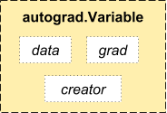
Self-grade module
PyTorch uses a technique called automatic differentiation. Namely, we have a recorder that records the operations we have performed and then plays them back to calculate our gradients. This technique is especially powerful when building neural networks, ya que ahorramos tiempo en una época al calcular la diferenciación de los parametersThe "parameters" are variables or criteria that are used to define, measure or evaluate a phenomenon or system. In various fields such as statistics, Computer Science and Scientific Research, Parameters are critical to establishing norms and standards that guide data analysis and interpretation. Their proper selection and handling are crucial to obtain accurate and relevant results in any study or project.... en la pasada directa.
Source: http://pytorch.org/about/
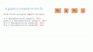
from torch.autograd import Variable

x = Variable(train_x)
y = Variable(train_y, requires_grad=False)
Optimal module
torch.optim is a module that implements various optimization algorithms used to build neural networks. Most of the most used methods are already supported, so we don't have to create them from scratch (Unless you want to!).
Below is the code to use an Adam optimizer:
optimizer = torch.optim.Adam(model.parameters(), lr=learning_rate)
modul nn
PyTorch autograd makes it easy to define computational graphics and take gradients, but the raw autograd may be too low a level to define complex neural networks. This is where the nn module can help.
The package nn defines a set of modules, which we can consider as a neural network layer that produces an output from the input and can have some trainable weights.
You can consider a module nn as the hard of PyTorch!
import torch

# define model
model = torch.nn.Sequential(
 torch.nn.Linear(input_num_units, hidden_num_units),
 torch.nn.ReLU(),
 torch.nn.Linear(hidden_num_units, output_num_units),
)
loss_fn = torch.nn.CrossEntropyLoss()
Now that you know the basic components of PyTorch, you can easily build your own neural network from scratch. Follow it if you want to know how!
Building a neural network in Numpy vs. PyTorch
I have mentioned above that PyTorch and Numpy are very similar. Lets see why. In this section, we will see an implementation of a simple neural network to solve a binary classification problem (you can read this article for detailed explanation).
## Neural network in numpy

import numpy as np

#Input array
X=np.array([[1,0,1,0],[1,0,1,1],[0,1,0,1]])

#Output
y=np.array([[1],[1],[0]])

#Sigmoid Function
def sigmoid (x):
 return 1/(1 + np.exp(-x))

#Derivative of Sigmoid Function
def derivatives_sigmoid(x):
 return x * (1 - x)

#Variable initialization
epoch=5000 #Setting training iterations
lr=0.1 #Setting learning rate
inputlayer_neurons = X.shape[1] #number of features in data set
hiddenlayer_neurons = 3 #number of hidden layers neurons
output_neurons = 1 #number of neurons at output layer

#weight and bias initialization
wh=np.random.uniform(size=(inputlayer_neurons,hiddenlayer_neurons))
bh=np.random.uniform(size=(1,hiddenlayer_neurons))
wout=np.random.uniform(size=(hiddenlayer_neurons,output_neurons))
bout=np.random.uniform(size=(1,output_neurons))

for i in range(epoch):
  #Forward Propogation
  hidden_layer_input1=np.dot(X,wh)
  hidden_layer_input=hidden_layer_input1 + bh
  hiddenlayer_activations = sigmoid(hidden_layer_input)
  output_layer_input1=np.dot(hiddenlayer_activations,road)
  output_layer_input= output_layer_input1+ bout
  output = sigmoid(output_layer_input)

  #Backpropagation
  E = y-output
  slope_output_layer = derivatives_sigmoid(output)
  slope_hidden_layer = derivatives_sigmoid(hiddenlayer_activations)
  d_output = E * slope_output_layer
  Error_at_hidden_layer = d_output.dot(wout.T)
  d_hiddenlayer = Error_at_hidden_layer * slope_hidden_layer
  wout += hiddenlayer_activations.T.dot(d_output) *lr
  bout += np.sum(d_output, axis=0,keepdims=True) *lr
  wh += X.T.dot(d_hiddenlayer) *lr
  bh + = np.sum(d_hiddenlayer, axis=0,keepdims=True) *lr

print('actual :n', Y, 'n')
print('predicted :n', output)
Now, try to spot the difference in a super simple implementation of the same in PyTorch (the differences are mentioned in bold in the following code).
## neural network in pytorch
import torch

#Input array
X = torch.Tensor([[1,0,1,0],[1,0,1,1],[0,1,0,1]])

#Output
y = torch.Tensor([[1],[1],[0]])

#Sigmoid Function
def sigmoid (x):
  return 1/(1 + torch.exp(-x))

#Derivative of Sigmoid Function
def derivatives_sigmoid(x):
  return x * (1 - x)

#VariableIn statistics and mathematics, a "variable" is a symbol that represents a value that can change or vary. There are different types of variables, and qualitative, that describe non-numerical characteristics, and quantitative, representing numerical quantities. Variables are fundamental in experiments and studies, since they allow the analysis of relationships and patterns between different elements, facilitating the understanding of complex phenomena.... initialization
epoch=5000 #Setting training iterations
lr=0.1 #Setting learning rate
inputlayer_neurons = X.shape[1] #number of features in data set
hiddenlayer_neurons = 3 #number of hidden layers neurons
output_neurons = 1 #number of neurons at output layer

#weight and bias initialization
wh=torch.randn(inputlayer_neurons, hiddenlayer_neurons).type(torch.FloatTensor)
bh=torch.randn(1, hiddenlayer_neurons).type(torch.FloatTensor)
road =torch.randn(hiddenlayer_neurons, output_neurons)
bout=torch.randn(1, output_neurons)

for i in range(epochEpoch es una plataforma que ofrece herramientas para la creación y gestión de contenido digital. Su enfoque se centra en facilitar la producción de multimedia, permitiendo a los usuarios colaborar y compartir información de manera eficiente. Con una interfaz intuitiva, Epoch se ha convertido en una opción popular entre profesionales y empresas que buscan optimizar su flujo de trabajo en la era digital. Su versatilidad la hace adecuada para diversas...):

  #Forward Propogation
  hidden_layer_input1 = torch.mm(X, wh)
  hidden_layer_input = hidden_layer_input1 + bh
  hidden_layer_activations = sigmoid(hidden_layer_input)

  output_layer_input1 = torch.mm(hidden_layer_activations, road)
  output_layer_input = output_layer_input1 + bout
  output = sigmoid(output_layer_input1)

  #Backpropagation
  E = y-output
  slope_output_layer = derivatives_sigmoid(output)
  slope_hidden_layer = derivatives_sigmoid(hidden_layer_activations)
  d_output = E * slope_output_layer
  Error_at_hidden_layer = torch.mm(d_output, wout.t())
  d_hiddenlayer = Error_at_hidden_layer * slope_hidden_layer
  wout += torch.mm(hidden_layer_activations.t(), d_output) *lr
  bout += d_output.sum() *lr
  wh += torch.mm(X.t(), d_hiddenlayer) *lr
  bh += d_output.sum() *lr

print('actual :n', Y, 'n')
print('predicted :n', output)
Comparison with other deep learning libraries
In one benchmarking script, se ha demostrado con éxito que PyTorch supera a todas las demás bibliotecas importantes de aprendizaje profundo en el trainingTraining is a systematic process designed to improve skills, physical knowledge or abilities. It is applied in various areas, like sport, Education and professional development. An effective training program includes goal planning, regular practice and evaluation of progress. Adaptation to individual needs and motivation are key factors in achieving successful and sustainable results in any discipline.... de una red de memoria a largo y corto plazo (LSTM) al tener la medianThe median is a statistical measure that represents the central value of a set of ordered data. To calculate it, the data is organized from lowest to highest and the number in the middle is identified. If there are an even number of observations, the two core values are averaged. This indicator is especially useful in asymmetric distributions, since it is not affected by extreme values.... de tiempo más baja por época (refer to the picture below).

APIs for data loading are well designed in PyTorch. Interfaces are specified in a data set, a sampler and a data loader.
When comparing tools for data loading in TensorFlow (readers, colas, etc.), I found PyTorchData loading modules are quite easy to use. What's more, PyTorch is perfect when trying to build a neural network, so we don't have to rely on third-party high-level libraries like keras.
Secondly, I still wouldn't recommend using PyTorch for implementation. PyTorch has yet to evolve. As the PyTorch developers have said, “What we are seeing is that users first create a PyTorch model. When they are ready to deploy their model into production, just turn it into a Caffe model 2 and then they send it to a mobile platform or another ".
Case study: Resolving an Image Recognition Problem in PyTorch
To get familiar with PyTorch, we will solve DataPeaker's deep learning practice problem: Identify the digits. Let's take a look at our problem statement:
Our problem is an image recognition problem, to identify digits of a given image of 28 x 28. We have a subset of images for training and the rest for testing our model.
First, download the train and test files. The dataset contains a compressed file of all images and both train.csv and test.csv are named after the corresponding train and test images. Additional features are not provided in the data sets, only raw images are provided in ‘.png’ format.
Let's start:
PASO 0: Getting ready
a) Import all necessary libraries
# import modules
%pylab inline
import os
import numpy as np
import pandas as pd
from scipy.misc import imread
from sklearn.metrics import accuracy_score
b) Let's set a seed value, so that we can control the randomness of our models
# To stop potential randomness
seed = 128
rng = np.random.RandomState(seed)
c) The first step is to set directory paths, For your safekeeping!
root_dir = os.path.abspath('.')
data_dir = os.path.join(root_dir, 'data')

# check for existence
os.path.exists(root_dir), os.path.exists(data_dir)
PASO 1: Data loading and preprocessing
a) Now let's read our data sets. These are in .csv formats and have a filename along with the corresponding tags.
# load dataset
train = pd.read_csv(os.path.join(data_dir, 'Train', 'train.csv'))
test = pd.read_csv(os.path.join(data_dir, 'Test.csv'))

sample_submission = pd.read_csv(os.path.join(data_dir, 'Sample_Submission.csv'))

train.head()
| file name | label | |
|---|---|---|
| 0 | 0.png | 4 |
| 1 | 1.png | 9 |
| 2 | 2.png | 1 |
| 3 | 3.png | 7 |
| 4 | 4.png | 3 |
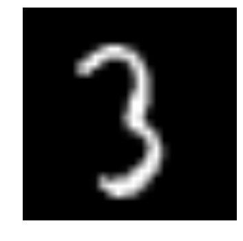
b) Let's see what our data looks like!! We read our image and show it.
# print an image
img_name = rng.choice(train.filename)
filepath = os.path.join(data_dir, 'Train', 'Images', 'train', img_name)

img = imread(filepath, flatten=True)

pylab.imshow(img, cmap='gray')
pylab.axis('off')
pylab.show()
d) For easier data manipulation, we store all our images as numpy arrays
# load images to create train and test set
temp = []
for img_name in train.filename:
  image_path = os.path.join(data_dir, 'Train', 'Images', 'train', img_name)
  img = imread(image_path, flatten=True)
  img = img.astype('float32')
  temp.append(img)

train_x = np.stack(temp)

train_x /= 255.0
train_x = train_x.reshape(-1, 784).astype('float32')

temp = []
for img_name in test.filename:
  image_path = os.path.join(data_dir, 'Train', 'Images', 'test', img_name)
  img = imread(image_path, flatten=True)
  img = img.astype('float32')
  temp.append(img)

test_x = np.stack(temp)

test_x /= 255.0
test_x = test_x.reshape(-1, 784).astype('float32')

train_y = train.label.values
e) How this is a typical AA problem, to test the correct operation of our model we create a validation set. Let's take a division size of 70:30 for the train set vs. the validation set
# create validation set
split_size = int(train_x.shape[0]*0.7)

train_x, val_x = train_x[:split_size], train_x[split_size:]
train_y, val_y = train_y[:split_size], train_y[split_size:]
PASO 2: Model building
a) Now comes the main part! Let's define our neural network architecture. We define a neural network with 3 input layers, hidden and exit. The number of input and output neurons is fixed, since the input is our image of 28 x 28 and the output is a vector of 10 x 1 what does the class represent. We take 50 neurons in the hidden layer. Here we use Adam like our optimization algorithms, which is an efficient variant of the Gradient Descent algorithm.
import torch
from torch.autograd import Variable
# number of neurons in each layer
input_num_units = 28*28
hidden_num_units = 500
output_num_units = 10

# set remaining variables
epochs = 5
batch_size = 128
learning_rate = 0.001
b) Time to train our model
# define model
model = torch.nn.Sequential(
  torch.nn.Linear(input_num_units, hidden_num_units),
  torch.nn.ReLU(),
  torch.nn.Linear(hidden_num_units, output_num_units),
)
loss_fn = torch.nn.CrossEntropyLoss()

# define optimization algorithm
optimizer = torch.optim.Adam(model.parameters(), lr=learning_rate)
## helper functions
# preprocess a batch of dataset
def preproc(unclean_batch_x):
  """Convert values to range 0-1"""
  temp_batch = unclean_batch_x / unclean_batch_x.max()

  return temp_batch

# create a batch
def batch_creator(batch_size):
  dataset_name="train"
  dataset_length = train_x.shape[0]

  batch_mask = rng.choice(dataset_length, batch_size)

  batch_x = eval(dataset_name + '_x')[batch_mask]
  batch_x = preproc(batch_x)

  if dataset_name == 'train':
    batch_y = eval(dataset_name).ix[batch_mask, 'label'].values

  return batch_x, batch_y
# train network
total_batch = int(train.shape[0]/batch_size)

for epoch in range(epochs):
  avg_cost = 0
  for i in range(total_batch):
    # create batch
    batch_x, batch_y = batch_creator(batch_size)

    # pass that batch for training
    x, y = Variable(torch.from_numpy(batch_x)), Variable(torch.from_numpy(batch_y), requires_grad=False)
    before = model(x)

    # get loss
    loss = loss_fn(pred, Y)

    # perform backpropagation
    loss.backward()
    optimizer.step()
    avg_cost += loss.data[0]/total_batch

  print(epoch, avg_cost)
# get training accuracy
x, y = Variable(torch.from_numpy(preproc(train_x))), Variable(torch.from_numpy(train_y), requires_grad=False)
before = model(x)

final_pred = np.argmax(pred.data.numpy(), axis=1)

accuracy_score(train_y, final_pred)
# get validation accuracy
x, y = Variable(torch.from_numpy(preproc(val_x))), Variable(torch.from_numpy(val_y), requires_grad=False)
before = model(x)
final_pred = np.argmax(pred.data.numpy(), axis=1)

accuracy_score(val_y, final_pred)
The training score turns out to be:
0.8779008746355685
while the validation score is:
0.867482993197279
This is quite an impressive score!, especially when we have trained a very simple neural network for only five epochs!
Final notes
I hope this article has given you an idea of how the PyTorch framework can change the perspective of building deep learning models. In this article, we just scratched the surface. To deepen, you can read the documentation Y tutorials on PyTorch's own official page.
In the next articles, i will apply PyTorch for audio analysis and we will try to create deep learning models for speech processing. Stay tuned!
Have you used PyTorch to build an application or in any of your data science projects? Let me know in the comments below..


