
This article was published as part of the Data Science Blogathon.
The Random Forest algorithm is without a doubt one of the most popular algorithms among data scientists.. Works great on both classification and regression problems. Random Forest is known as an ensemble technique because it is a collection of multiple decision trees.
What was the main purpose of using multiple decision trees?
Using a single decision tree has several drawbacks. When we use a single decision tree to solve a problem statement, we find a situation of low bias and high variance. Namely, el árbol capturará toda la información sobre los datos de trainingTraining is a systematic process designed to improve skills, physical knowledge or abilities. It is applied in various areas, like sport, Education and professional development. An effective training program includes goal planning, regular practice and evaluation of progress. Adaptation to individual needs and motivation are key factors in achieving successful and sustainable results in any discipline...., as well as the noise. As a result, the model developed using the decision tree algorithm will work well with the training data, but it will perform poorly when evaluated on the test data (unknown data). Overfitting is the condition of having a low bias and a high variance.
Decision tree -----> Overfit ————–> low deviation high variance
Random Forest uses multiple decision trees to avoid this problem present in the decision tree algorithm.
But, How does Random Forest address the problem of overfitting?
The Random Forest algorithm does not use all the training data when training the model, as seen in the diagram below. Instead, sample rows and columns with repetition. This means that each tree can only be trained with a limited number of rows and columns with repeating data. In the following diagram, training data 1 are used to train the decision tree 1, and training data n is used to train decision tree n. But nevertheless, since each tree is created to its full depth and has the property of overfitting, How do we avoid this problem?
Since the algorithm does not depend on the result of a particular decision tree. You will first get the results of all decision trees and then give the final result based on the type of statement of the problem. For instance; if the type of statement of the problem is the classification, majority voting would be used. suppose we are classifying “Yes” Y “no” with 10 trees, and 6 trees are sorting “Yes” Y 4 they are classifying “no”, the final answer will be “Yes” using majority voting. ¿Qué pasa si nuestra salida es una variableIn statistics and mathematics, a "variable" is a symbol that represents a value that can change or vary. There are different types of variables, and qualitative, that describe non-numerical characteristics, and quantitative, representing numerical quantities. Variables are fundamental in experiments and studies, since they allow the analysis of relationships and patterns between different elements, facilitating the understanding of complex phenomena.... continuous? Then, el resultado final sería la media o la medianThe median is a statistical measure that represents the central value of a set of ordered data. To calculate it, the data is organized from lowest to highest and the number in the middle is identified. If there are an even number of observations, the two core values are averaged. This indicator is especially useful in asymmetric distributions, since it is not affected by extreme values.... de la producción de todos los árboles.
Classification problem -> Majority voting
Regression problem -> Media / Median
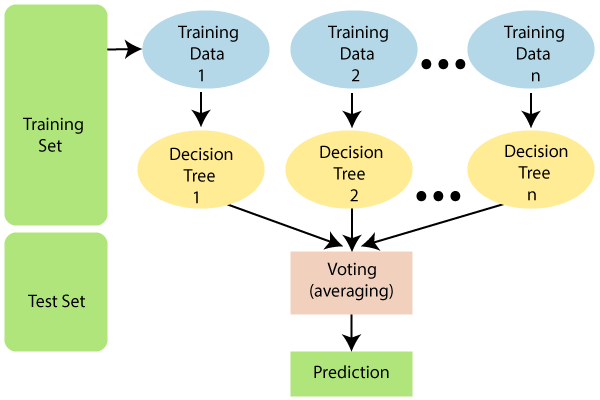
The model performs row sampling. But nevertheless, Characteristics sampling should be done according to the type of problem statement.
- If the problem statement type is “classification”.
The total number of features / random columns selected = p ^ ½ or the square root of p,
where p is the total number of Independent attributes / characteristics present in the data.
- If the problem statement type is “regression”.
The total number of random columns selected = p / 3.
Random Forest avoids overfitting with: –
1) Performing Row and Characteristic Sampling.
2) Connecting all decision trees in parallel.
Why is it known as the Bootstrap Aggregation technique?
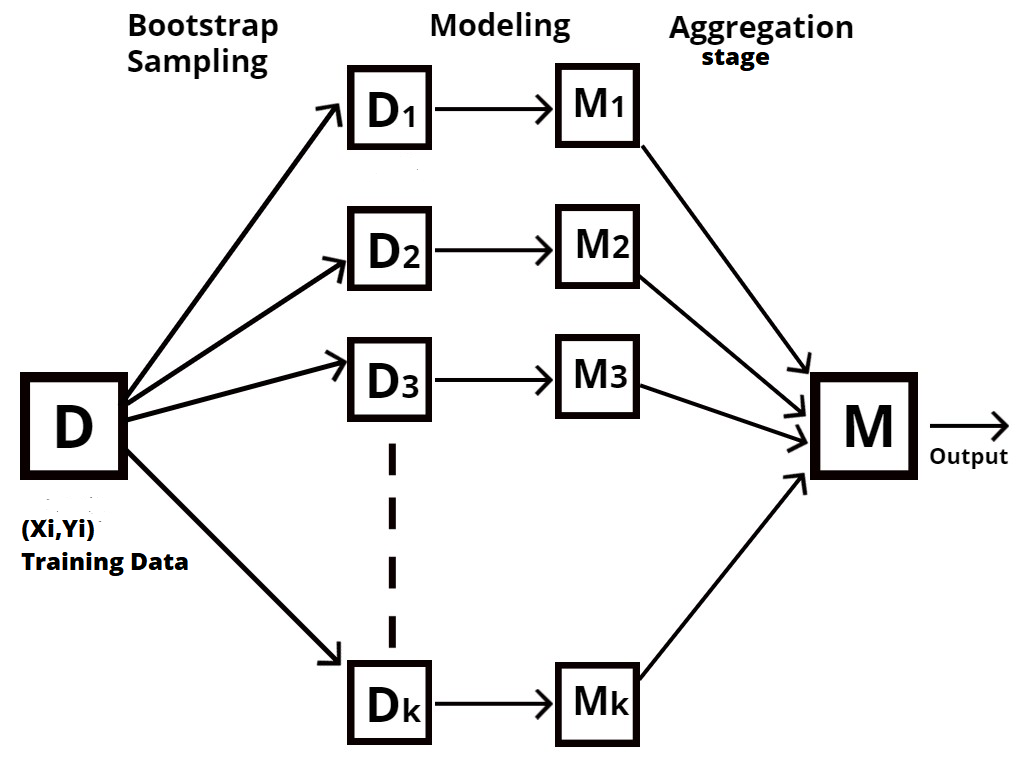
Random Forest is a type of set technique, also known as bootstrap aggregation O harpillera.
The process of sampling different rows and characteristics of the training data with repetition to build each decision tree model is known as bootstrapping., as shown in the following diagram.
Aggregation is the process of taking all the results from each decision tree and combining them to produce a final result using majority votes or average values., according to the type of statement of the problem.
Random forest using R
library(caTools)

library(randomForest)
We need to install the libraries' caTools’ y ‘randomForest’ and activate them using the library function ()
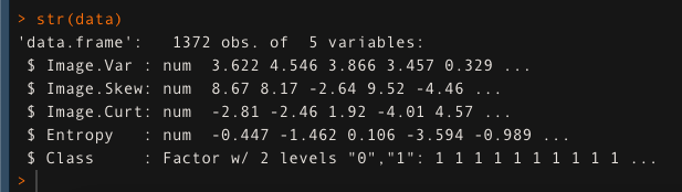
We have used the banknote authentication data set and stored it in the variable 'data'. We will check the structure of the data using the str function ().
data <- read.csv ('bank_note_data.csv', header = T)
str (data)
Now we will divide our data into test and train parts. 80% for training and 20% to test the model.
seeds (123)
split <- sample.split (data, SplitRatio = 0.8)
train <- subset (data, divide == T)
proof <- subset (data, division == F)
After dividing the data, we will build our model using the randomForest function (). Here ‘ntree’ is the hyperparameter. what needs to be adjusted. In this case, is selected as 500.
random_model <- random_forest (Class ~., data = train, mtry = 2, ntree = 500)
Predicting Model Accuracy on Test Data Using Prediction Function ().
eval <- predict (random_model, proof)
Evaluate the precision of the model using the confusion matrix.
confusionMatrix (table (eval, proof $ Class))
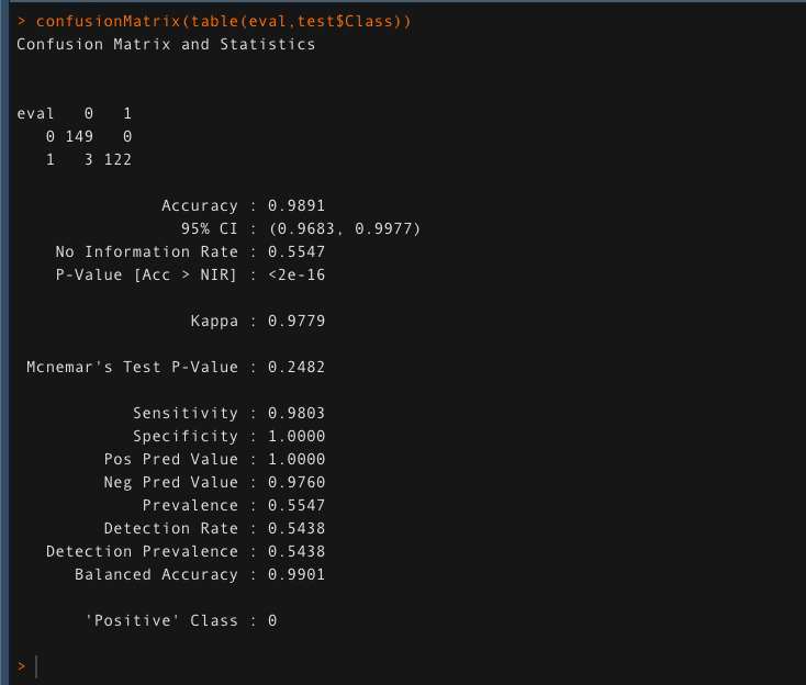
The model gives an accuracy of 98,91% in the test data. This ensures that Random Forest is doing a fantastic job..





