
This post was made public as part of the Data Science Blogathon
Introduction
sampling to obtain the probability of a range of an unknown quantity. Sounds difficult! do not worry, we will explore this in depth in this post
A brief history:
The Monte Carlo Method was invented by John Neumann and Ulam Stanislaw to drive decision making under uncertain conditions. It is named after a well-known Monte Carlo casino town called Monaco, since the element of chance is central to the modeling approach, since it is similar to a roulette game.
In simple words, Monte Carlo simulation is a method of estimating the value of a unknown quantity with the help of inferential statistics. You do not need to delve into inferential statistics to have a solid understanding of how Monte Carlo simulation works. Despite this, this post will only go through those points of inferential statistics that will be relevant to us in the Monte Carlo simulation.
Inferential statistics is responsible for the population what is our set of examples and sample, which is a suitable subset of the population. The key point to pay attention is that a random sample tends to exhibit the same features / property as the population from which it is extracted.
We will see an example to understand how the Monte Carlo simulation works.
Our goal is to estimate how likely we are to get ahead if we flip a coin an infinite number of times..
1. Say we flip it once and go ahead. Are we safe to say that our answer is 1?
2. Now we flipped the coin again and the face reappeared. Are we sure that the next release will also be ahead?
3. We flip it over and over, Let's say 100 times, and strangely the head appears every time. Now, Do we have to accept the fact that the next turn will result in another head?
4. Let's change the scene and suppose that 100 releases, 52 resulted in the head resting, 48 they became crosses. The probability that the next pitch will hit the head is 52/100? Given the observation, is our best estimate, but confidence will remain low.
Why is there a difference in the confidence level?
It is essential to know that our estimate depends on two things
1. Size: The size of the sample (as an example, 100 vs 2 In the cases 2 Y 4 respectively)
2. Difference: sample variance (all results as head vs. 52 heads as in the case 3 Y 4 respectively)
3. As the variance of the observation increases (cases 3 Y 4), the need arises for a more extensive observation (as in the cases 2 Y 4) to have the same degree of confidence.
Now we will be simulating a game of roulette (python):
Roulette is a game in which a disk with blocks (half red and half black) in which a ball can be contained, spin with a ball. We need to guess a number and if the ball lands on this number, then it's a win, and we won an amount of (amount paid for a slot
) X (no. Total slots on the machine).
Roulette class():
    def __init__(self):
        self.pockets = []
        for i in range(1,37):
            self.pockets.append(i)
        self.ball = None
        self.pocketOdds = len(self.pockets) - 1
Def Spin(self):
    self.ball = random.choice(self.pockets)
def betPocket(self, Pocket, AMT):
    if str(Pocket) == str(self.ball):
        return amt*self.pocketOdds
    else: return -amt
def __str__(self):
        return 'Fair Roulette'
def playRoulette(game, numSpins, Pocket, Bet):
    totPocket = 0
    for i in range(numSpins):
        game.spin()
    totPocket += game.betPocket(Pocket, Bet)
    if toPrint:
        print (numSpins, 'spins of', game)
        print ('Expected return betting', Pocket, '=',
            str(100*totPocket/numSpins) + '%n')
    return (totPocket/numSpins)
game = Roulette()
for numSpins in (100, 1000000):
    for i in range(3):
        playRoulette(game, numSpins, 5, 1, True)
100 Roulette Spins
Expected Return Bets 5 = -100.0%
100 Roulette Spins
Expected Return Bets 5 = 42.0%
100 Roulette Spins
Expected Return Bets 5 = -26.0%
1000000 Roulette Spins
Expected Return Bets 5 = -0,0546%
1000000 Roulette Spins
Expected Return Bets 5 = 0,502%
1000000 Roulette Spins
Expected Return Bets 5 = 0,7764%
Law of Large Numbers
On repeated independent tests with the population's constant probability p of a particular result on each test, the probability of the outcome occurring, In other words, obtained from samples. Differs of p Converges to Zero As the the number of trials goes to infinity.
It simply means that if deviations occur (variance) expected behavior (probability p), these deviations are likely to be offset in the future by the opposite deviation.
Now let's talk about an interesting incident that took place on 18 August 1913, in a Monte Carlo casino. At roulette, black climbed a record twenty-six times in a row, and panic arose to bet on red (to equal deviation from expected behavior)
Let's analyze this situation mathematically
1. Probability 26 consecutive reds = 1 / 67,108,865
2. Probability 26 consecutive reds when 25 previous scrolls were red = 1/2
Regression to the mean
1. After an extreme random event, the next random event is likely to be less extreme, so that the mean is kept.
2. As an example, if the roulette wheel is spun 10 times and the reds come every time, then it is an extreme event = 1/1024 and it is likely that in the next 10 turns we get less than 10 red, but the average number is 5 only.
Then, when we look at the mean of 20 turns, will be closer to the expected mean of 50% of red than of 100% in the first 10 turns.
Now is the time to face some reality.
Sample space of possible results
1. It is not feasible to guarantee perfect precision through sampling and it cannot be said that an estimate is not exactly correct..
We are faced with a question here: How many samples does it take to look at before we can have significant confidence in our answer?
It depends on the variability in the underlying distribution.
Confidence levels and confidence intervals
Just like in a real life situation, we cannot be sure of any unknown parameter obtained from a sample for the entire population, so we use confidence levels and confidence intervals.
The confidence interval provides a range in which the unknown value is likely to be contained with the confidence that the unknown value is strictly within that range..
As an example, the performance of betting on a slot machine 1000 times in roulette is -3% with a marginMargin is a term used in a variety of contexts, such as accounting, Economics and printing. In accounting, refers to the difference between revenue and costs, which allows the profitability of a business to be evaluated. In the publishing field, The margin is the white space around the text on a page, that makes it easy to read and provides an aesthetic presentation. Its correct management is essential.. of error of +/- 4% with a confidence level of 95%.
It can be further decoded as we run an infinite test of 1000,
Average performance / expected average would be -3%
Performance would vary roughly between + 1% Y -7% that besides the 95% of the times.
Probability density function (PDF).
The general shape distribution is established through the probability density function (PDF). It is established as the probability that the variableIn statistics and mathematics, a "variable" is a symbol that represents a value that can change or vary. There are different types of variables, and qualitative, that describe non-numerical characteristics, and quantitative, representing numerical quantities. Variables are fundamental in experiments and studies, since they allow the analysis of relationships and patterns between different elements, facilitating the understanding of complex phenomena.... is between a.
The area under the curve between the two PDF points is the probability that the random variable is within that range.
Let's conclude our learning with an example:
Let's say there is a deck of shuffled cards and we need to find the probability of getting 2 consecutive kings if they place the cards in the order they are laid.
Analytical method:
P (at least 2 consecutive kings) = 1-P (no consecutive kings)
= 1- (49! X 48!) / ((49-4)! X52!) = 0.217376
By Monte Carlo simulation:
Steps
1. Select random data points repeatedly: here we assume that the shuffling of the cards is random
2. Performing deterministic calculations. Several of these shuffle and find the results.
3. Combine the results: Exploring the result and ending with our conclusion.
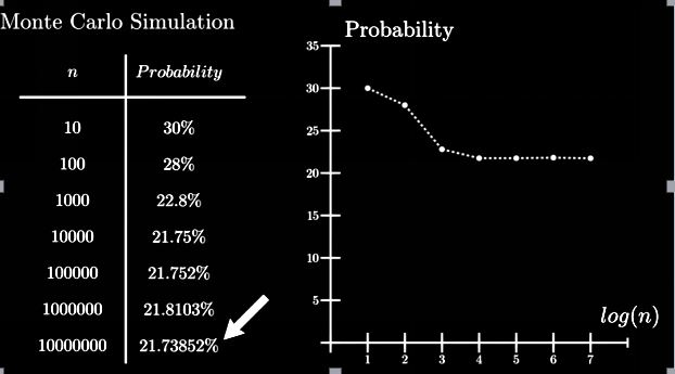
Through the Monte Carlo method we achieve an almost exact solution from the analytical method.
Advantages of Monte Carlo simulation
- Easy to implement and provides statistical sampling for numerical experiments using the computer.
- Provides us with satisfactory approximate solutions to computationally expensive mathematical problems.
- Can be used for both deterministic and stochastic problems.
Disadvantages of Monte Carlo simulation
- Sometimes it takes a long time, since we have to generate a large number of samples to obtain the desired satisfactory result.
- The results obtained with this method are only the approximation of the true answer and not the exact answer.
About the Author
Soy Dinesh Junjariya, a Btech student from IIT Jodhpur.
For any suggestion, comment below.
The media shown in this post is not the property of DataPeaker and is used at the author's discretion.





