Monte Carlo simulation | Perform Monte Carlo simulation in R

This article was published as part of the Data Science Blogathon.

Introduction

This article aims to present the Monte Carlo simulation for the analysis of variable uncertainty. Monte Carlo can replace error propagation because it overcomes the disadvantages of error propagation. we will discuss:

• How to propagate the error;
• Why use Monte Carlo instead of error propagation? Y
• The steps to realize the Monte Carlo uncertainty.

Let's start this discussion with simple things. How much does a City A employee spend on living expenses in a month? There are thousands of employees in city A with different living expenses. To answer the previous question, we must ask several employees and record their responses. Those employees will respond differently. Your living expenses will vary in a probability distribution. Although we do not have the resources to ask all employees, we can sample a group of, for instance, 50 employees so that the survey represents the population.

But nevertheless, we still need a number to represent the total living expense. Let's say we get that the average monthly living expense is $ 2000. O well, another way is to use the median to represent total spending. To express other possible living expenses, we can use the standard deviation. For instance, monthly living expenditure in city A is $ 2000 ± 500 (mean ± standard deviation).

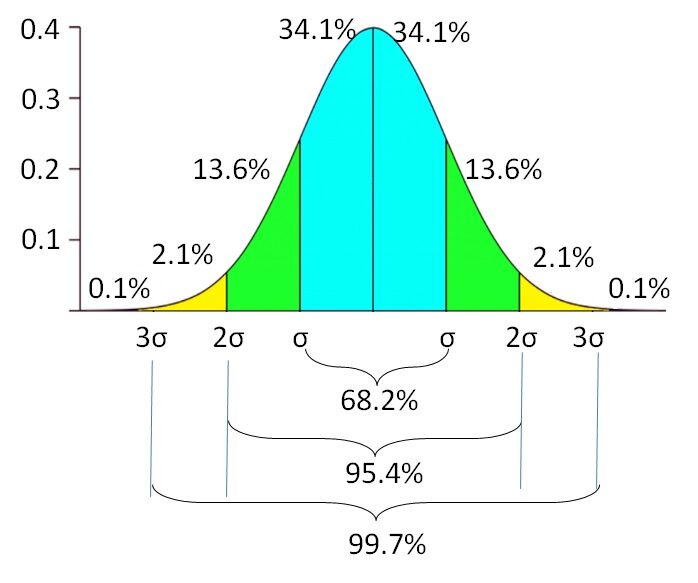
It means that if the data is normally distributed, the 68,2% of employees spend between $ 1500 Y $ 2500. There is another 31,8% of employees who spend less than $ 1500 and more of $ 2500 in monthly living costs. The probability of life expense decreases as it moves away from the average. There is a probability of 0,1% of finding employees with living expenses less than $ 500 the superior to $ 3500. The standard deviation reflects the variable uncertainty of the life expense. Indicates the lower and upper extent of the variable, instead of relying on a single value.

Error propagation

Since city A employees have income: $ 3200 ± 2000, living expenses: $ 2000 ± 500, credit: $ 180 ± 130, unexpected income or expenses: $ 20 ± 300 and bank interest rate: 0,85 ± 0,35% monthly. We want to calculate how much an employee can save in a month. The equation is expressed below:

Savings = (Income – Living expenses – Credit + Income / unexpected expenses) × (1 + Interests)

Monthly savings are calculated as total income deducted from living expenses and credit and added to unexpected income or expenses.. After one month, nominal saving increases due to bank interest. We will calculate the average monthly savings and the uncertainty. Look at the following equation on how to calculate the uncertainty.

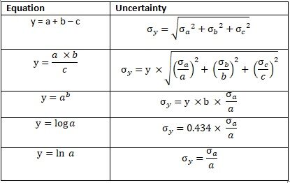
Fig. 2 Error propagation

Saving1 = ((3200 ± 2000) - (2000 ± 500) - (180 ± 130) + (20 ± 300)) × (1 + (0.0085 ± 0.0035))

Saving1 = 1040 ± σSaving_1

σSaving_1 = ((20002 + 5002 + 1302 + 20002))0.5

σSaving_1 = 2087

Saving1 ± σSaving_1 = 1040 ± 2087

This calculates the monthly savings after accounting for bank interest.

Saving = Saving1 × (1 + (0.0085 ± 0.0035)) 

Saving = (1040 ± 2087) × (1.0085 ± 0.0035)

Saving = 1049 ± σSaving_2

σSaving = 1049 × ((2087/1040)2 + (0.0035/1.0085)2)0.5

σSaving = 1049 × 2.01

σSaving = 2105

Savings ± σ_Saving = 1049 ± 2105

From the result, we can see that, on average, people can save $ 1049 in a month with the uncertainty of $ 2105. The lower limit of monthly savings is – $ 1056 ($ 1049 – $ 2105), what is a negative value. The uncertainty itself is 2105, What is it 2 times greater than the mean value. If we visualize the graph, we can see that employee savings range from – $ 6000 Y $ 8000. It seems strange because the lower and upper limits are almost balanced. I think that, in reality, the amount of savings should have a greater variability than the amount of the deficit.

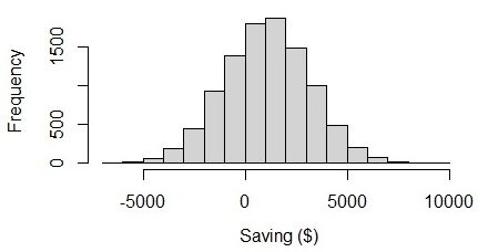
Fig. 3 Visualization of savings in a normal distribution

How is this happening? The problem is in the income data. The income of $ 3200 ± 2000 has high uncertainty due to income variability. The uncertainty is more than a third of the mean value. If we assume that this is a normal distribution, we will see that the 4.8% of the population have incomes below 0, what doesn't seem likely to happen. In fact, income must always be above% 0. This problem occurs when we assume that all variables are normally distributed, but in reality they are not.

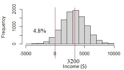
Fig. 4 Normal distribution if the standard deviation of income is too large

Monte Carlo simulation

What is the solution? Another way to evaluate uncertainty is by applying the Monte Carlo simulation. Monte Carlo is originally the name of an administrative area in Monaco. But the Monte Carlo in our discussion today is statistical stuff.. Monte Carlo can overcome the downside of error propagation. The Monte Carlo simulation, as opposed to error propagation, can work on a data distribution other than the normal distribution and on data with a large standard deviation.

Fig. 5 Monte Carlo in Monaco. Source: Google Map

Monte Carlo simulation simulates or generates a set of random numbers according to the data distribution and the parameters of each variable. Once generated, all the values ​​of the variables are calculated using the equation. This sounds a bit more complicated than using error propagation. But use data science tools, like Python or R, it will be very simple. In this discussion, we will demonstrate the use of the statistical language R.

Steps to perform a Monte Carlo simulation

1. Check the probability density function of the data distribution.

Let's say we examine the data record provided by the survey of 50 surveyed. There are many types of probability density functions and we have to determine which one fits our data. Variables with normal distribution are only living expenses and unexpected income or expenses. The distribution of income data is positive.

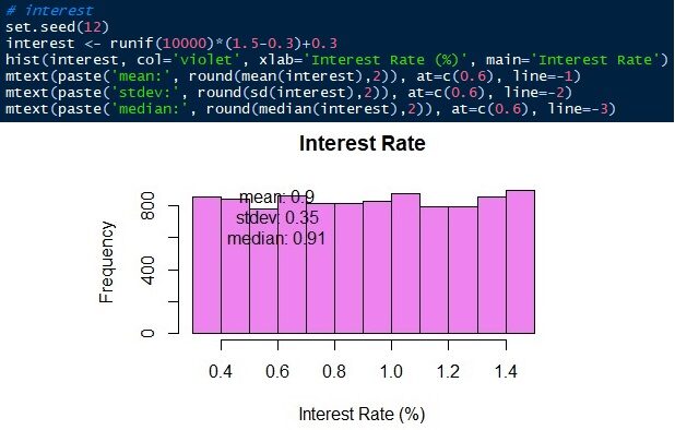
In this case, we will treat it as a gamma distribution. This is why the mean and spread of the error are not suitable for this data.. The other two variables do not have a normal distribution either.. The bank interest rate is evenly distributed between 0,3 Y 1,5.

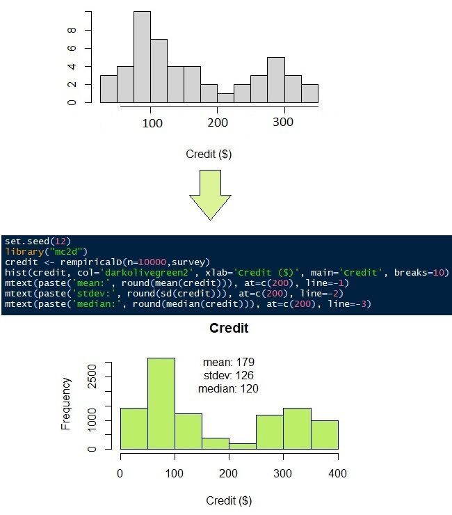
The distribution of data on loans to pay off credit is quite unique. The data are mainly distributed in two population groups. The first group has less credit than the second. Let's say that the distribution of credit data does not fit any probability density function. Later, we will use a nonparametric distribution.

2. Generate Monte Carlo simulation

Generating Monte Carlo simulation means generating a set of random numbers with the same data distribution as the original data. To do this, we simply set the number of simulations and the distribution parameters according to the type of distribution. We set the number of simulations to 10,000. It means that we will simulate the data of 50 surveyed in 10,000 data.

The parameters of the normal distribution are mean / mean and standard deviation. We know that the means ± standard deviations of living expenses and unexpected income or results are 2000 ± 500 Y 20 ± 300 respectively. Now, we can generate the distributions. In this article, I will use the R language. Of course, other data science languages, like Python, they can do it too. See that the simulated data has a similar mean and standard, not the same, than input parameters.

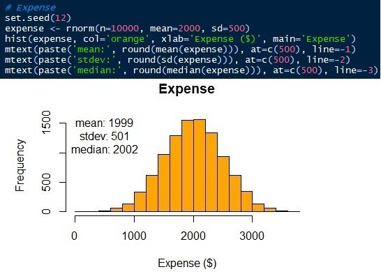
Fig. 6 Normal distribution of living expenses

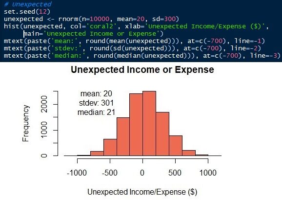
Fig. 7 Normal distribution of unexpected income or expenses

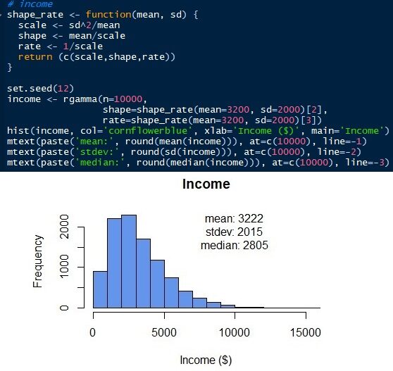
To generate the gamma distribution, we need to know other parameters. Unlike the normal distribution, the gamma distribution has scale, shape and speed as parameters. But we can get those parameters with the mean and standard deviation (of). Scale = sd²/to mean. Shape = medium / scale. Rate = 1 / scale. Later, we can simulate the gamma distribution of employee income as shown below. The gamma distribution can only have positive values. There is no value below 0 since the income of all employees must be a positive number. The normal distribution would give negative values ​​if the standard error is too large. See that the simulated distribution has a mean and standard deviation of 3222 Y 2015 respectively, that are close to the original input parameters. But we have a median of 2805. The median of the gamma distribution, unlike normal distribution, is far from average.

The credit to pay monthly, as mentioned earlier, does not have a proper probability density function. Take a look at the answers from 50 surveys in Figure 9 (gray histogram). It seems that most people have to pay off their credit from $ 100 Y $ 300. To simulate the 50 observations in 10,000 observations, we can use a nonparametric distribution. As its name suggests, nonparametric distribution requires no parameters, as average, the standard deviation, the form or the rate, as the normal and gamma distributions do. Requires only the original data.

The last variable to simulate is the bank interest rate. The bank interest rate varies from 0,3 a 1,5 uniformly. Let's do the same 10,000 observations ranging from 0.3 a 1.5 with the same probability.

3. Combination of Monte Carlo simulations

The last step is to combine the Monte Carlo Simulations using the equation to calculate the monthly savings. To do this, we just need to put all simulations together in one table. Later, we can calculate 10,000 monthly savings rows. The result is $ 1073 ± 2052, not much different from the propagation of the error. But, Monte Carlo simulation shows probability density. We can see that the median savings is $ 666 and the data ranges between $ 2000 Y 10000.

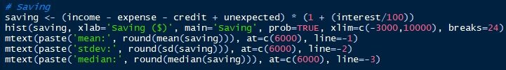
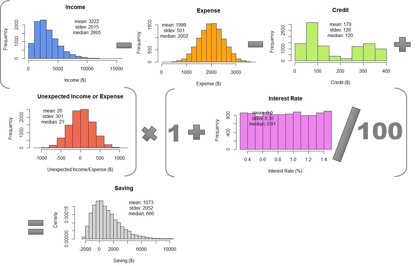
Table 1 – Combination of Monte Carlo simulations

Now, let's look at another example with spatial and temporal variability. The task is to calculate the surface runoff of a basin. The basin is the limit of surface water hydrology. All the rain that falls below the basin will not cross out of the boundary. Part of the rain infiltrates the soil according to the size of the soil particles and the type of land cover. Water that does not infiltrate the soil is called surface runoff. Surface runoff will flow into the river as river discharge.

The following table shows the monthly rainfall intensity in a year and the runoff coefficient in a 1,5 km.² cuenca. The uncertainty may be due to spatial and temporal heterogeneity. The coefficient of precipitation and runoff (due to soil and land cover type) varies spatially in the basin. Basin precipitation is measured with various rain gauges. They give mean rainfall with uncertainty due to spatial distribution. The land cover distribution also gives the uncertainty of the runoff coefficient.

A runoff coefficient is the proportion of rainfall that does not infiltrate the soil and becomes surface runoff. The forest or thick soil type has a low runoff coefficient. Settlements or houses have a high runoff coefficient. Conversion of forest land cover to settlements increases the runoff coefficient because a higher proportion of rainwater will be surface runoff.

Temporal variability also occurs because the rains in the wet and dry seasons are different.. The change in land cover over time also causes the temporal variability of the runoff coefficient. Other sources of uncertainty are the quality of the measurement tools, measurement methods, environmental conditions and other unexplained conditions due to lack of knowledge.

My	Rainfall (mm / my)	Runoff coefficient	Area (km2)
one	320 ± 37	0,3 ± 0,2	1,5
feb	350 ± 59	0,3 ± 0,2	1,5
mar	205 ± 26	0,4 ± 0,1	1,5
Apr	170 ± 41	0,4 ± 0,1	1,5
Mayo	106 ± 48	0,4 ± 0,1	1,5
jun	91 ± 32	0,4 ± 0,1	1,5
jul	77 ± 16	0,4 ± 0,1	1,5
ago	52 ± 15	0,7 ± 0,2	1,5
sep	100 ± 50	0,7 ± 0,2	1,5
oct	120 ± 46	0,7 ± 0,2	1,5
nov	253 ± 45	0,7 ± 0,2	1,5
Dec	210 ± 48	0,7 ± 0,2	1,5

The equation is surface runoff = rainfall intensity × runoff coefficient × basin area. The entire distribution is simulated using a gamma distribution. Average monthly surface runoff is 124.000 ± 30 m³/my. The median is 120.000 m³/my.

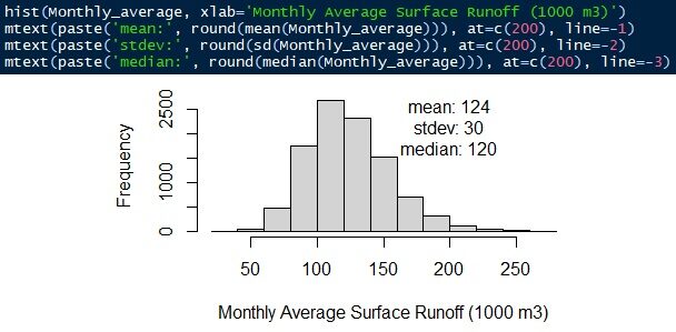
Fig. 12 Average monthly surface runoff

About the Author

Connect with me here https://www.linkedin.com/in/rendy-kurnia/

Related