
This article was published as part of the Data Science Blogathon.
Introduction
The main objectives of validating a model include testing the conceptual soundness of the model and continuous fit to purpose., including identification of potential risks and limitations. These tests must constitute an effective challenge to the existing production model for the benefit of its improvement., risk mitigation. The data for this exercise are taken from here.
Validation framework
The following tests were performed to validate the results of the model:
- Model variables: IV, linearity and VIF
- 3. Model fit: AUROC graphics, Gini, KS and gain and lift
- 4. Model tests: sensitivity analysis
- 5. Stability coefficient: signal stability and coefficient stability
2.1 Data checks
Dependent variables
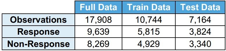
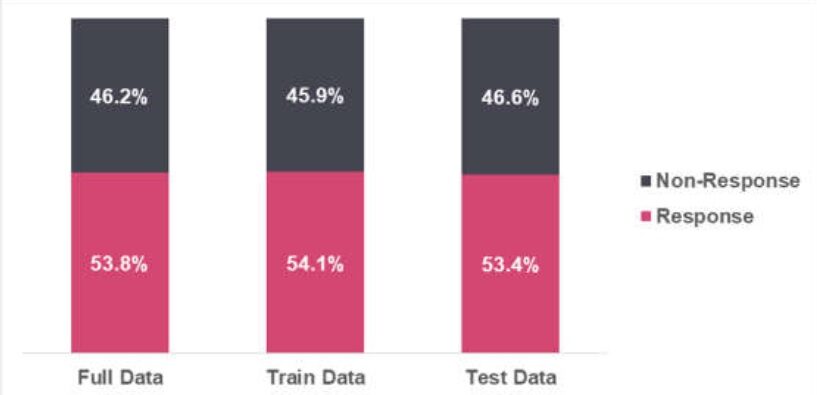
It is observed that the response distribution (Y = 1) and no answer (Y = 0) it is very similar between full data, train data and test data.
· The answer (Y = 1) indicates that the applicant has applied for the loan
· Unanswered (Y = 0) indicates that the applicant has not applied for the loan
Independent variables
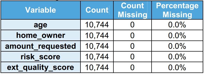
Independent variables include personal and financial information. Risk scores are used to develop the model. There is 5 independent variables in the model.
It is observed that there are no missing values in the train data set.
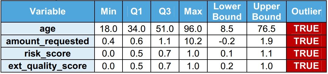
It is observed that there are outliers in the train data set. The range between quartiles (IQR = Q3 – Q1) is used to identify the points of sale. Outliers are values greater than the upper limit (Q1 + 1,5 x IQR) or values lower than the lower limit (Q1 – 1,5 x IQR). The validation team recommends that outliers be addressed before developing the model.
2.2. Model variables
Information value (IV)
from statsmodels.stats.outliers_influence import variance_inflation_factor
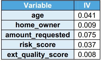
The explanatory power of the variableIn statistics and mathematics, a "variable" is a symbol that represents a value that can change or vary. There are different types of variables, and qualitative, that describe non-numerical characteristics, and quantitative, representing numerical quantities. Variables are fundamental in experiments and studies, since they allow the analysis of relationships and patterns between different elements, facilitating the understanding of complex phenomena.... is captured using IV. As the explanatory power of the variable increases, increases IV. It is observed that all the variables have IV <0.1, indicating that they have low explanatory power in the train data set.
Linearity
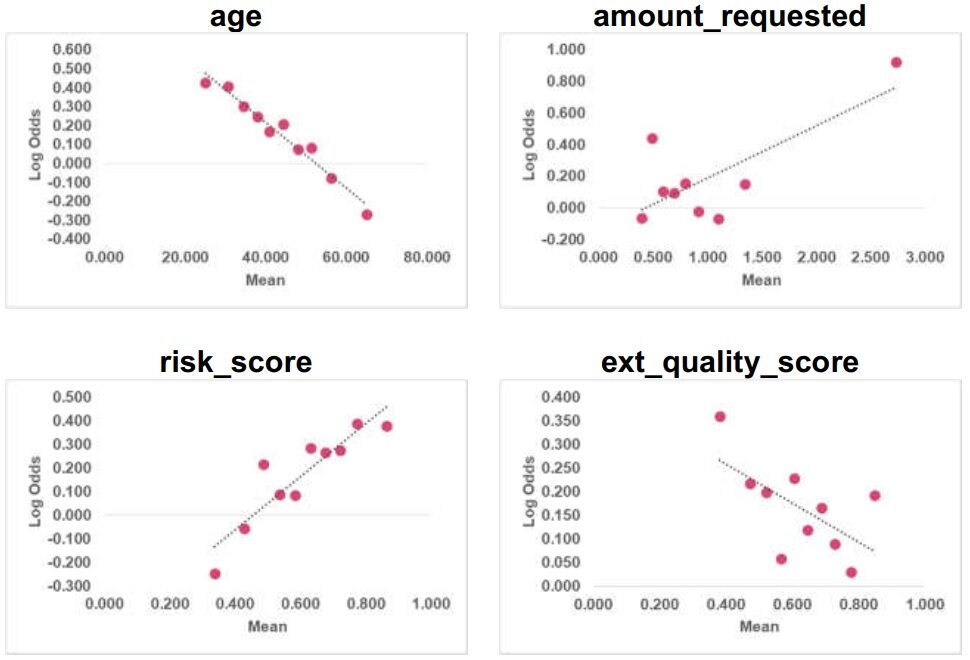
Paso 1: make 10 containers for each numeric variable
Paso 2: for each interval, compute the mean of the variable and the corresponding log probabilities
The linearity of the numerical variables is checked (age, requested amount, risk_score and quality_score_ ext) in the train data. it is observed that it acts & risk_score son lineales y amount_requested & ext_quality_score no son lineales. The validation team recommends that the transformations be tested to obtain a linear relationship.
Variance information factor (LIVELY)
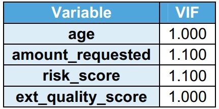
VIF indicates multicollinearity between independent variables. It is observed that its VIF is less than 2 in the dataset of trainingTraining is a systematic process designed to improve skills, physical knowledge or abilities. It is applied in various areas, like sport, Education and professional development. An effective training program includes goal planning, regular practice and evaluation of progress. Adaptation to individual needs and motivation are key factors in achieving successful and sustainable results in any discipline..... VIF less than 2 indicates no multicollinearity. Home_owner is a flag, Thus, not considered for VIF.
2.3 Model fit
AU-ROC
sklearn.metrics.auc(x, Y)
The area under the receiver operator curve (AUROC) is used to measure the predictive power of the model. AUROC = 0,50 indicates that there is no predictive power and AUROC = 1,00 indicates perfect predictive power. Model developed with train data is run with test data and full data. It is observed that there is no significant deviation in the AUROC values.
It is observed that AUROC is less than 0,6. This indicates that the model does not have good predictive power.. The validation team recommends using additional variables to improve the fit of the model..

Gini
Formula: Gini = 2 x AUROC – 1
Gini se deriva de AUROC. Gini = 0.0 indicates that there is no predictive power and Gini = 1.0 indicates perfect predictive power. Model developed with train data is run with test data and full data. It is observed that there is no significant deviation in the Gini values.

Kansas
scipy.stats.ks_2samp
The Kolmogorov-Smirnov test (KS) measures the separation between the cumulative% of events and the cumulative% of no events. It is observed that the statistics of the KS tests are lower than 40, which indicates that the model is not capable of separating events and non-events.

Gain and elevation graphs
Paso 1: Calculate the probability of each observation.
Paso 2: Rank these probabilities in decreasing order.
Paso 3: Construct deciles with each group having almost the 10% of the observations.
Paso 4: Calculate the response rate in each decile for Good (responders), A little (non-responders) and total.
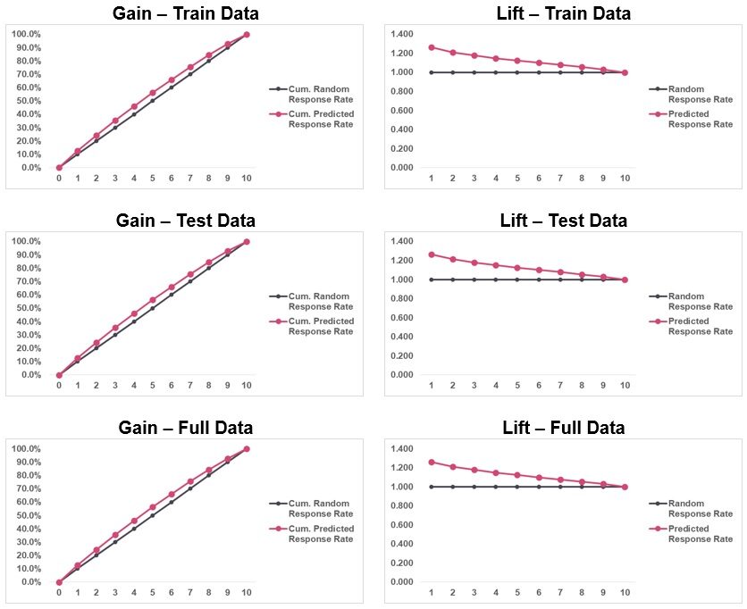
Gain and elevation graphs are data visualization tools that compare the classifier's ability to capture response rate. It is observed that the predicted cumulative response rate is very close to the cumulative random response rate. Indicates that the model has low predictive power. The validation team recommends using additional variables to improve the fit of the model..
2.4 Model tests
Sensitivity analysis
Paso 1: normalize all variables
Paso 2: run the logistic regression between the dependent variable and the first
Paso 3: run the logistic regression between the dependent variable and the second
Paso 4: repeat the previous step for the rest of the variables
Paso 5: the coefficient of the variable indicates the sensitivity between the variable and the logarithmic probabilities of the dependent variable
The sensitivity of the model with respect to the independent numerical variables is tested. Sensitivity is checked on the train data. The objective of this exercise is to identify the most sensitive variables. It is observed that age and risk_score are the most sensitive variables and ext_quality_score is the least sensitive variable.

2.5. Coefficient stability
Coefficient stability
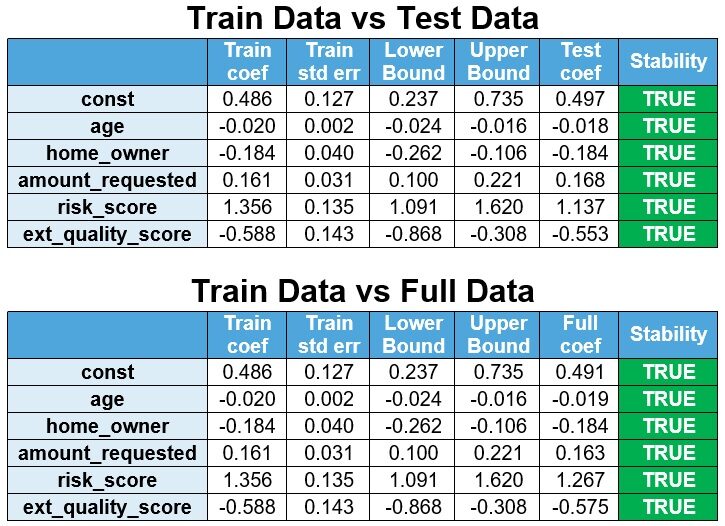
The model is re-estimated from the test data and the full data and the coefficients are compared to the train data. If the coefficients of the reestimated model are within the confidence interval of the 95% (Train coefficient ± 1,96 x Err std de tren), then the coefficients are stable.
The lower limit is defined as Train Coef – 1,96 x Err std of train and the upper limit is defined as Coef of train + 1,96 x Err std de tren. It is observed that the coefficients are stable.
Signal stability
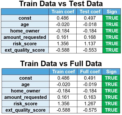
The model is re-estimated from the test data and the full data and the coefficients are compared to the train data.
Signs are observed to be stable.
Conclution
Validation found the model to be stable. But nevertheless, three serious findings have been raised:
· Finding 1 (input data) – It is observed that there are outliers in the train data set. The validation team recommends that outliers be addressed before developing the model.
· Finding 2 (input data) – Note that amount_requested & ext_quality_score no son lineales. The validation team recommends that the transformations be tested to obtain a linear relationship.
· Outcome 3 (model fit) – AUROC is observed to be low, Gini is low and KS is low, which indicates that the model is not capable of separating events and non-events. The validation team recommends using additional variables to improve the fit of the model..
The media shown in this article is not the property of DataPeaker and is used at the author's discretion.





