Decision tree classification | Decision Tree Classification Guide
Contents
Overview
What is the Decision Classification Tree Algorithm?
How to build a decision tree from scratch
Decision Tree Terminologies
Difference between random forest and decision tree
Decision Trees Python Code Implementation
There are several algorithms in machine learning for regression and classification problems, but opting for The best and most efficient algorithm for the given data set is the main point to make while developing a good machine learning model..
One of these algorithms good for classification problems / categorical and regression is the decision tree
Decision trees generally implement exactly human thinking ability when making a decision, so it's easy to understand.
The logic behind the decision tree can be easily understood because it shows a flowchart type structure / tree-like structure that makes it easy to view and extract information from the background process.
Table of Contents
What is a decision tree?
Decision tree elements
How to make a decision from scratch
How does the decision tree algorithm work?
Knowledge of EDA (exploratory data analysis)
Decision trees and random forests
Advantages of Decision Forest
Disadvantages of Decision Forest
Python code implementation
1. What is a decision tree?
A decision tree is a supervised machine learning algorithm. Used in both classification and regression algorithms.. The decision tree is like a tree with nodes. The branches depend on several factors. Splits the data into branches like these until it reaches a threshold value. A decision tree consists of the root nodes, child nodes and leaf nodes.
Let's understand the decision tree methods by taking a real life scenario
Imagine that you play soccer every Sunday and you always invite your friend to play with you. Sometimes, your friend comes and others don't.
The factor of coming or not depends on numerous things, like the weather, the temperature, wind and fatigue. We started to take all of these characteristics into consideration and started to track them along with your friend's decision to come play or not..
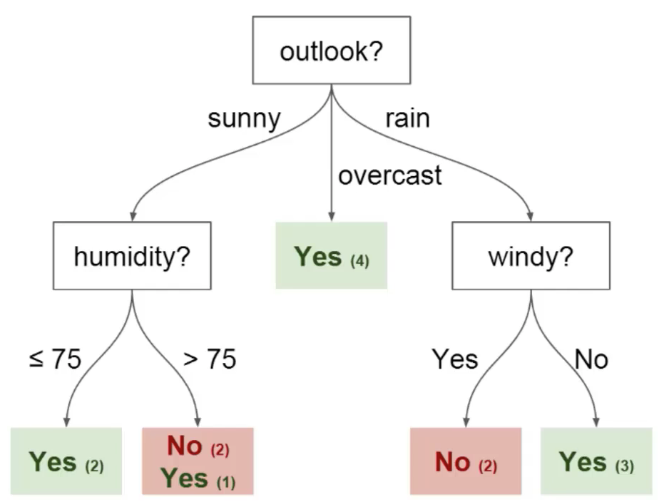
You can use this data to predict whether your friend will come to play soccer or not. The technique you could use is a decision tree. This is what the decision tree would look like after deployment:
2. Elements of a decision tree
Each decision tree consists of the following list of elements:
a nodeNodo is a digital platform that facilitates the connection between professionals and companies in search of talent. Through an intuitive system, allows users to create profiles, share experiences and access job opportunities. Its focus on collaboration and networking makes Nodo a valuable tool for those who want to expand their professional network and find projects that align with their skills and goals....
b Edges
c Root
d Leaves
a) Nodes: It is the point where the tree is divided according to the value of some attribute / dataset characteristic.
b) Edges: It directs the result of a split to the next node that we can see in the figure"Figure" is a term that is used in various contexts, From art to anatomy. In the artistic field, refers to the representation of human or animal forms in sculptures and paintings. In anatomy, designates the shape and structure of the body. What's more, in mathematics, "figure" it is related to geometric shapes. Its versatility makes it a fundamental concept in multiple disciplines.... previous that there are nodes for features such as perspective, humidity and wind. There is an advantage for each potential value of each of those attributes / features.
c) Root: This is the node where the first division takes place.
d) Leaves: These are the terminal nodes that predict the outcome of the decision tree.
3. How to build decision trees from scratch?
When creating a decision tree, the main thing is to select the best attribute from the list of total characteristics of the dataset for the root node and for the subnodes. The selection of the best attributes is achieved with the help of a technique known as measureThe "measure" it is a fundamental concept in various disciplines, which refers to the process of quantifying characteristics or magnitudes of objects, phenomena or situations. In mathematics, Used to determine lengths, Areas and volumes, while in social sciences it can refer to the evaluation of qualitative and quantitative variables. Measurement accuracy is crucial to obtain reliable and valid results in any research or practical application.... attribute selection (ASM).
With the help of ASM, we can easily select the best characteristics for the respective decision tree nodes.
There are two techniques for ASM:
a) Information gain
b) IndexThe "Index" It is a fundamental tool in books and documents, which allows you to quickly locate the desired information. Generally, it is presented at the beginning of a work and organizes the contents in a hierarchical manner, including chapters and sections. Its correct preparation facilitates navigation and improves the understanding of the material, making it an essential resource for both students and professionals in various areas.... by Gini
a) Information gain:
1Information gain is the measurement of changes in entropy value after division / segmentationSegmentation is a key marketing technique that involves dividing a broad market into smaller, more homogeneous groups. This practice allows companies to adapt their strategies and messages to the specific characteristics of each segment, thus improving the effectiveness of your campaigns. Targeting can be based on demographic criteria, psychographic, geographic or behavioral, facilitating more relevant and personalized communication with the target audience.... dataset based on an attribute.
2 Indicates how much information a feature provides us / attribute.
3 Following the value of information gain, node division and decision tree construction are underway.
The decision tree 4 always tries to maximize the value of the information gain, and a node / attribute that has the highest value of the information gain is divided first. Information gain can be calculated using the following formula:
Information Gain = Entropy (S) – [(Weighted Avg) *Entropy(each feature)
Entropy: Entropy signifies the randomness in the dataseta "dataset" or dataset is a structured collection of information, which can be used for statistical analysis, Machine learning or research. Datasets can include numerical variables, categorical or textual, and their quality is crucial for reliable results. Its use extends to various disciplines, such as medicine, economics and social science, facilitating informed decision-making and the development of predictive models..... It is being defined as a metric to measure impurity. Entropy can be calculated as:
Entropy(s)= -P(yes)log2 P(yes)- P(no) log2 P(no)
Where"WHERE" is a term in English that translates as "where" in Spanish. Used to ask questions about the location of people, Objects or events. In grammatical contexts, it can function as an adverb of place and is fundamental in the formation of questions. Its correct application is essential in everyday communication and in language teaching, facilitating the understanding and exchange of information on positions and directions....,
S= Total number of samples
P(yes)= probability of yes
P(no)= probability of no.
b) Gini Index:
Gini index is also being defined as a measure of impurity/ purity used while creating a decision tree in the CART(known as Classification and Regression Tree) algorithm.
An attribute havingThe verb "have" In Spanish it is a fundamental auxiliary that is used to form compound tenses. Its conjugation varies according to time and subject, being "I", "You", "has", "we have", "You" Y "have" The Forms of the Present. What's more, in some regions, Used "have" as an impersonal verb to indicate existence, like in "there is" to "there is/are". Its correct use is essential for effective communication in Spanish.... a low Gini index value should be preferred in contrast to the high Gini index value.
It only creates binary splits, and the CART algorithm uses the Gini index to create binary splits.
Gini index can be calculated using the below formula:
Gini Index= 1- ∑jPj2
Where pj stands for the probability
4. How Does the Decision Tree Algorithm works?
The basic idea behind any decision tree algorithm is as follows:
1. SelectThe command "SELECT" is fundamental in SQL, used to query and retrieve data from a database. Allows you to specify columns and tables, filtering results using clauses such as "WHERE" and ordering with "ORDER BY". Its versatility makes it an essential tool for data manipulation and analysis, facilitating the obtaining of specific information efficiently.... the best Feature using Attribute Selection Measures(ASM) to split the records.
2. Make that attribute/feature a decision node and break the dataset into smaller subsets.
3 Start the tree-building process by repeating this process recursively for each child until one of the following condition is being achieved :
a) All tuples belonging to the same attribute value.
b) There are no more of the attributes remaining.
c ) There are no more instances remaining.
5. Decision Trees and Random Forests
Decision trees and Random forest are both the tree methods that are being used in Machine Learning.
Decision trees are the Machine Learning models used to make predictions by going through each and every feature in the data set, one-by-one.
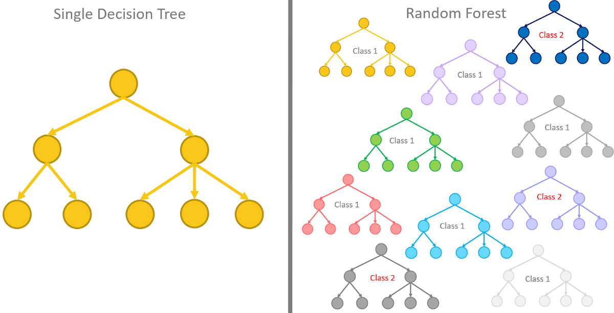
Random forests on the other hand are a collection of decision trees being grouped together and trained together that use random orders of the features in the given data sets.
Instead of relying on just one decision tree, the random forest takes the prediction from each and every tree and based on the majority of the votes of predictions, and it gives the final output. In other words, the random forest can be defined as a collection of multiple decision trees.
6. Advantages of the Decision Tree
1 It is simple to implement and it follows a flow chart type structure that resembles human-like decision making.
2 It proves to be very useful for decision-related problems.
3 It helps to find all of the possible outcomes for a given problem.
4 There is very little need for data cleaning in decision trees compared to other Machine Learning algorithms.
5 Handles both numerical as well as categorical values
7. Disadvantages of the Decision Tree
1 Too many layers of decision tree make it extremely complex sometimes.
2 It may result in OverfittingOverfitting, or overfitting, It's a phenomenon in machine learning where a model fits too closely with the training data, capturing irrelevant noise and patterns. This results in poor performance on unseen data, since the model loses generalization capacity. To mitigate overfitting, Techniques such as regularization can be used, cross-validation and reduction of model complexity.... ( which can be resolved using the Random Forest algorithm)
3 For the more number of the class labels, the computational complexity of the decision tree increases.
8. Python Code Implementation
#Numerical computing libraries
import pandas as pd
import numpy as np
import matplotlib.pyplot as plt
import seaborn as sns
# Divida el conjunto de datos en datos de trainingTraining is a systematic process designed to improve skills, physical knowledge or abilities. It is applied in various areas, like sport, Education and professional development. An effective training program includes goal planning, regular practice and evaluation of progress. Adaptation to individual needs and motivation are key factors in achieving successful and sustainable results in any discipline.... y datos de prueba
from sklearn.model_selection import train_test_split
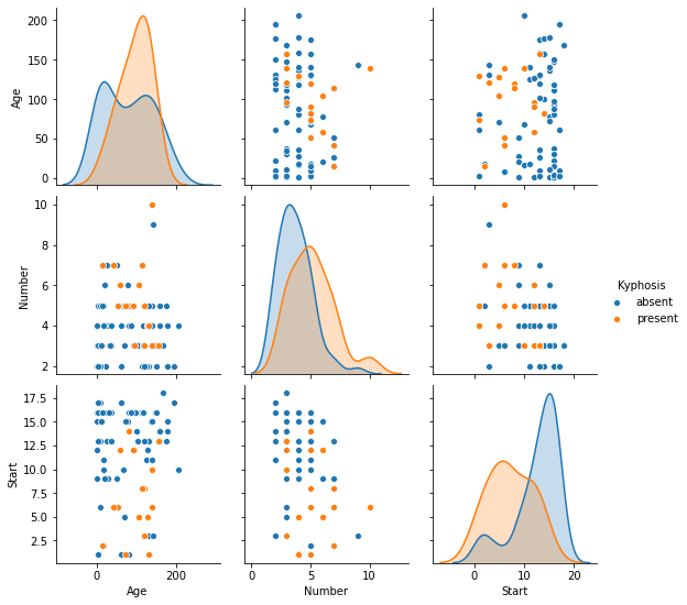
x = raw_data.drop('Kyphosis', axis = 1)
y = raw_data['Kyphosis']
x_training_data, x_test_data, y_training_data, y_test_data = train_test_split(x, Y, test_size = 0.3)
#Train the decision tree model
from sklearn.tree import DecisionTreeClassifier
model = DecisionTreeClassifier()
model.fit(x_training_data, y_training_data)
predictions = model.predict(x_test_data)
# Measure performance of the decision tree model
from sklearn.metrics import classification_report
from sklearn.metrics import confusion_matrix
print(classification_report(y_test_data, predictions))
print(confusion_matrix(y_test_data, predictions))
With this I end this blog. Hi everyone, Namaste My name is Pranshu Sharma and i'm a data science enthusiast
Thank you very much for taking your valuable time to read this blog.. Feel free to point out any errors (after all, i am an apprentice) and provide the corresponding comments or leave a comment.
Dhanyvaad !! Feedback: Email: [email protected]
The media shown in this DataPeaker article is not the property of DataPeaker and is used at the Author's discretion.