Overview
- Advanced Excel charts are a great way to create effective and impactful stories for our audience..
- Learn it 3 advanced Excel charts here to impress your manager and build rapport with your stakeholders
Introduction
I was completely focused on analyzing data and using statistical methods to build complex data science models when I started my analytical journey.. In fact, I know that many newcomers are obsessed with this method of approaching things. I have some news for you: in reality, this is not the core quality of a good analyst.
Stakeholders couldn't understand what you were trying to communicate to them. There was a missing link across the stage: the narration.
I was able to level up by improving my storytelling skills. To pass the story on to our management team, a key skill to learn is understanding different types of charts. As usual, podemos explicar la mayoría de las cosas con un bar graphicThe bar chart is a visual representation of data that uses rectangular bars to show comparisons between different categories. Each bar represents a value and its length is proportional to it. This type of chart is useful for visualizing and analyzing trends, facilitating the interpretation of quantitative information. It is widely used in various disciplines, such as statistics, Marketing and research, due to its simplicity and effectiveness.... simple o un Dispersion diagramThe scatter plot is a graphical tool used in statistics to visualize the relationship between two variables. It consists of a set of points in a Cartesian plane, where each point represents a pair of values corresponding to the variables analyzed. This type of chart allows you to identify patterns, Trends and possible correlations, facilitating data interpretation and decision-making based on the visual information presented...., but they don't always satisfy the need.
There is no one-size-fits-all chart and that's why, to create intuitive visualizations, it is imperative that we understand the different types of graphics and their use. And Excel is the perfect tool for creating powerful yet powerful charts for our analytics audience..
In this article, I am going to discuss 3 powerful and important advanced Excel charts that will make you a pro in front of your audience (and even your manager).
This is the sixth article in my Excel for Analysts series. I highly recommend reading the previous articles to become a more efficient analyst.:
I encourage you to check out the resources below if you are a beginner to Excel and Business Analytics:
Table of Contents
- Excel advanced charts n. ° 1: sparklines
- Excel advanced charts n. ° 2: gantt charts
- Excel advanced charts n. ° 3 – Thermometer charts
Excel advanced charts n. ° 1: sparklines
I'll start with one of my favorite chart types: sparkline graphics. These graphics really help me create amazing dashboards!! Then, What are sparklines?
Sparklines are typically small in size and fit into a single cell. These charts are wonderful for visualizing trends in your data., such as seasonal increase or decrease in value.
In Microsoft Excel, have 3 different types of minigraphs: line, column and gain / lost. Let's see how we can make a sparkline with this problem statement:
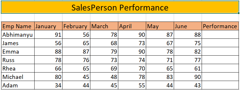
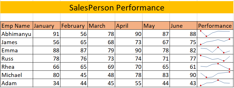
You are an analyst in a product-based company and you want to understand the performance of salespeople during the first six months of the year. Decide to use sparklines for this.
Follow the steps or watch the video to better understand sparklines:
Paso 1: choose your sparkline type
You will first need to select the type of sparkline you want to plot. In our case, usaremos un line graphThe line chart is a visual tool used to represent data over time. It consists of a series of points connected by lines, which allows you to observe trends, Fluctuations and patterns in the data. This type of chart is especially useful in areas such as economics, Meteorology and scientific research, making it easier to compare different data sets and identify behaviors across the board...
Go to Insert -> Line:
Paso 2: create minigraphs
Select the first row of the data in the Data range and the corresponding Location range:
We have successfully made our Sparkline chart!! Now we just need to drag it for all our rows:
Paso 3: desired format
We have the basic sparklines ready. We can format it so that the graph is more intuitive to understand. In this case, we selected Decisive point Y Low point:
Finally, our table looks like this:
Try using sparklines in your reports next time. You'll love it!
Excel advanced charts n. ° 2: gantt charts
If you have previously worked in the field of project management, must be familiar with Gantt charts. These charts are one of the most popular and useful ways to track project activities over time..
Gantt charts are essentially bar charts. Each activity represents a bar. The length of the bar represents the duration of the activity or task.
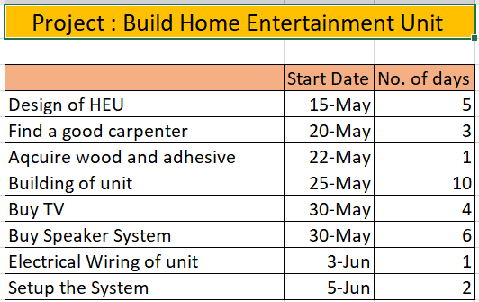
To understand Gantt charts, Let's consider a statement of the problem. There are two roommates: Joey y Chandler. Due to the recent pandemic, they usually stay at home and decide to build themselves a home entertainment unit. El interés de Chandler en la analyticsAnalytics refers to the process of collecting, Measure and analyze data to gain valuable insights that facilitate decision-making. In various fields, like business, Health and sport, Analytics Can Identify Patterns and Trends, Optimize processes and improve results. The use of advanced tools and statistical techniques is essential to transform data into applicable and strategic knowledge.... y la visualización convierte este pequeño proyecto en una representación de diagrama de Gantt. Lets see how.
You can refer to the video or steps below as per your convenience:
Paso 1: select the stacked bar chart
Since Gantt charts are basically bar charts, let's first select one:
Go to Insert -> 2D bar -> Stacked grouped bar
Paso 2: put the categories in reverse order
You may notice that the sequence of events is actually opposite to the required sequence. So let's reverse it.
Select the categories on the axis and right click -> Go to Axis Format:
Now just select the checkbox – “Categories in reverse order”:
Paso 3: make date bar chart invisible
If you look at the graph correctly, you will notice that the blue graphic represents the start date. We will remove the color from this chart to get the desired Gantt chart.
Select the blue chart -> the right button of the mouse ->Format the data series:
Now go to the fill section and select – Unfilled:
Now the graph looks like this:
Paso 4: select minimum and maximum limits
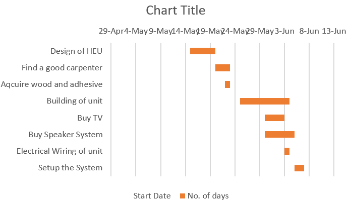
The date in our chart begins on 29 of April, what we clearly don't want, as it uses unnecessary space. Then, let's select the limits for the dates of our Gantt chart.
Select the date (horizontal axis) -> The right button of the mouse -> Format axis:
Now we simply need to provide a minimum and maximum deadline:
We have made the following table:
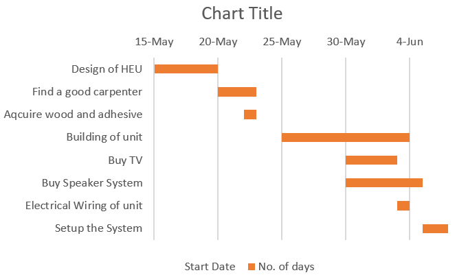
Paso 5 – Format your chart
We have created our Gantt chart, but we won't show it to anyone unless it looks attractive to the eye, so we will format a bit to make our diagram look good.
Here we have done some things:
- Removed shaft
- Changed the title and
- Tick marks added
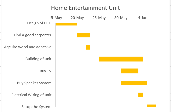
Congratulations! You have created your first Gantt chart!! Joey and Chandler must be enjoying their new entertainment unit.
Excel advanced charts n. ° 3 – Thermometer charts
Thermometer charts are really cool and distribute crucial information in a very neat way. These charts are great for visualizing actual value and target value.. It is useful to visualize sales, step on the website, etc. Let's better understand the graphs with a problem statement.
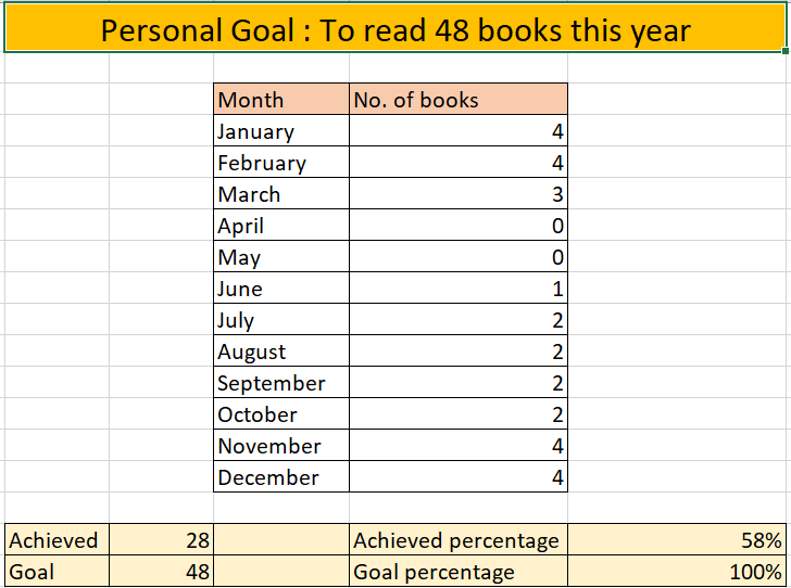
Every new year, people tend to make a decision. Jake había tomado la resolutionThe "resolution" refers to the ability to make firm decisions and meet set goals. In personal and professional contexts, It involves defining clear goals and developing an action plan to achieve them. Resolution is critical to personal growth and success in various areas of life, as it allows you to overcome obstacles and keep your focus on what really matters.... de completar 48 books during the year. That's around 1 book per week. Let's understand how Jake acted.
You can follow the steps and refer to the video to understand it better:
Paso 1: select grouped graphics
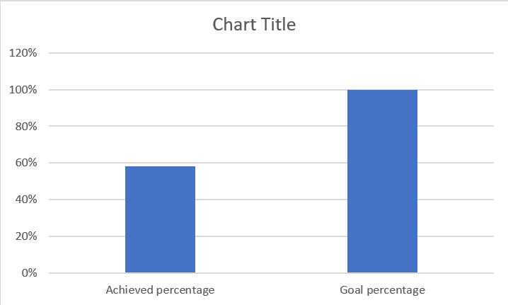
Select the percentage data as shown below:
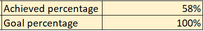
Go to Insert -> 2D column -> Grouped column:
Here is our graph:
Paso 2: combine column
Go to Graphic design -> Select Change row / column and click OK:

Now, right click on the Accomplished % column -> Go to Format string -> To select Secondary shaft:
This will overlap both columns in one column.
Paso 3: select minimum and maximum
We have our columns overlapping but on different axes, so let's give it a uniform limit.
Select the percentages (vertical axis values) and right click -> Format axis:
Now select the minimum limit as 0.0 and the maximum limit as 1.0:
Paso 3: format the chart
Select the Target % chart and right click -> Format the data series:
Go to Fill options -> To select Unfilled Y Solid line border:
Now we have a table that finally looks like a thermometer table. All we need is an additional format.
Here, we have followed the steps below to format:
- Remove grid lines
- Rearrange the chart size
- Give the title of the chart
- Add tick marks
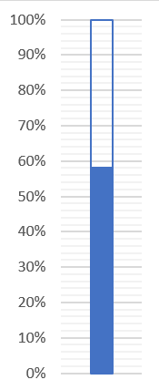
Perfect!
Final notes
In this article, we cover three beautiful excel charts of different types to help you become an efficient analyst. Hope these graphics help you create amazing visualizations and save you a lot of time. and impress your boss. 🙂
Let me know your favorite Excel charts that you think make for a great visualization.


