Introduction
Machine learning algorithms are classified into three types: supervised learning, unsupervised learning and reinforced learning. K-means clustering is an unsupervised machine learning technique. When the output or response variable is not provided, this algorithm is used to categorize the data into different groups to better understand it. Also known as a data-driven machine learning approach, as it groups data based on hidden patterns, knowledge and similarities in data.
Consider the following diagram: if you are asked to group the people in the picture into different groups or groups and you don't know anything about them, will certainly try to locate the qualities, characteristics or physical attributes that these people share. After observing these people, it is concluded that they can be segregated based on their height and width; since you have no prior knowledge about these people. K-means clustering performs roughly equivalent work. Try to classify the data into groups based on similarities and hidden patterns. “K” in clustering of K-means refers to the number of clusters that the algorithm will generate in the data.
K-Means grouping: How does it work?
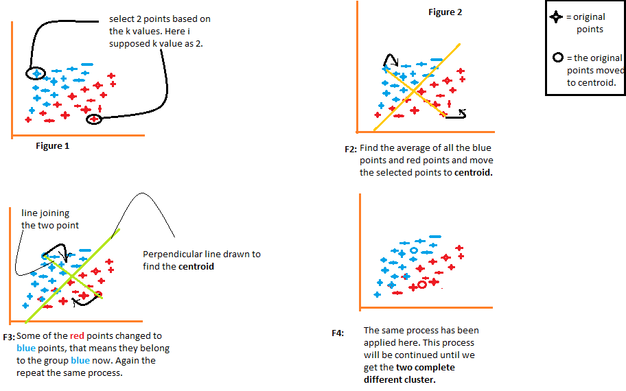
1) The algorithm arbitrarily chooses the number k of centroids, as indicated in the figure 1 from the following diagram. Where k is the number of clusters that the algorithm would create. Let's say we want the algorithm to create two groups from the data, so we will set the value of k to 2.
2) Then group the data into two parts using the distances calculated from both centroids., as illustrated in Figure 2. The distance of each point from both centroids is calculated individually and later it will be added to the group of that centroid with which the distance is calculated. shorter.
The algorithm also draws a line joining the centroids and a perpendicular line that tries to group the data into two groups.
3) Once all the data points are grouped based on their minimum distances from the corresponding centroids, the algorithm calculates the mean of each group. Then the mean and centroid values of each group are compared. If the centroid value differs from the mean, then the centroid is shifted to the mean value of the group. Both the centroid “Red” As the “blue” are relocated to the mean of the group in the figure 3 from the following diagram.
Group the data once more using these updated centroids. Due to the change in the positions of the centroids, some data points can now be shifted in the other group.
4) Again, calculates the mean and compares it with the centroid of the newly generated groups. If both are different, the centroid will be relocated back to the group mean. This process of calculating the mean and comparing it to the centroid is repeated until the values of the centroid and the mean are equal. (centroid value = group mean). This is the point at which the algorithm has segmented the data into 'K groups’ (2 in this case).
How to find out what is the optimal value of k?
The first step is to provide a value for k. Each subsequent step executed by the algorithm is completely dependent on the specified value of k. This value of k helps the algorithm determine the number of clusters to generate. This emphasizes the importance of providing the precise value of k. Here, a method known as the “elbow method” to determine the correct value of k. This is a graph of ‘Number of clusters K’ versus “Total within the sum of the square”. Discrete values of k are plotted on the x-axis, while the sums of squares of the groups are plotted on the y-axis.
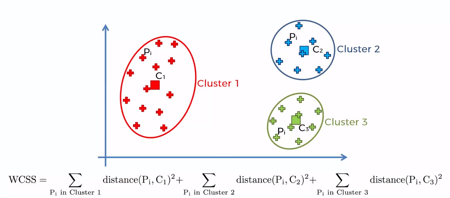
The sum of the squared distances between the individual points and the centroid in each group, followed by the sum of the squared distances for all clusters, It is called "Sum of squares within the cluster". You will be able to understand this with the help of the following steps.
1) Calculate the distance between the centroid and each point in the group, square and then add the squared distances for all points in the group.
2) Calculate the sum of the squared distances of the remaining groups in the same way.
3) Finally, add all the sums of groups to obtain the value of the "Sum of the square within the group" as shown in the following figure.
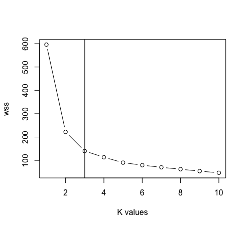
The “total within the sum of the square” begins to decrease as the value of k increases. The graph between the number of clusters and the total within the sum of squares is shown in the following figure. The optimal number of clusters, or the correct value of k, is the point at which the value begins to slowly decrease; this is known as the “elbow point”, and the elbow point in the following graph is k = 4. The “Elbow method” it is named for the similarity of the graph to the elbow, and the optimal point for “k” is the elbow point .
Advantages of k-means clustering
1) Tagged data is not mandatory. Since a lot of real world data is not labeled, as a result, are frequently used in a variety of real-world problem statements.
2) It is easy to implement.
3) Can handle massive amounts of data.
4) When the data is big, work faster than hierarchical grouping (for k little ones).
Disadvantages of K-means clustering
1) The value of K must be selected manually using the “elbow method”.
2) The presence of outliers would have an adverse impact on grouping. As a result, outliers must be removed before using k-means grouping.
3) Groups do not intersect; a point can only belong to one group at a time. As a result of the lack of overlap, certain points are placed in wrong groups.
K-means grouping with R
- We will import the following libraries into our work.
library (intercalation)
library (ggplot2)
library (dplyr)
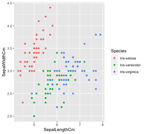
- We will work with the iris data, containing three classes: “Iris-silky”, “Iris-versicolor” e “Iris-virginica”.
data <- read.csv ("iris.csv", header = T)
- Let's see how these three classes are related to each other. The species “Iris-versicolor” (verde) e “Iris-verginica” (blue) they are not linearly separable. As you can see in the graph below, they intermingle.
data%>% ggplot (aes (SepalLengthCm, SepalWidthCm, color = Species)) +
geom_point ()
- After removing the species column from the data. Now we will use the graph of the elbow method between “Sum of squares within the cluster” Y “K values” to determine the appropriate value of k. K = 3 is the best value for k in this case (Note: there is 3 classes in the original iris data, which guarantees the precision of the value of k).
data <- data[, -5]
maximum <- 10
scal <- scale (data)
wss <- sapply (1: maximum, function (k) {kmeans (scal, k, nstart = 50, iter.max = 15) $ tot.withinss})
plot (1: max, wss, type = “b”, xlab = “k values”)
abline (v = 3)
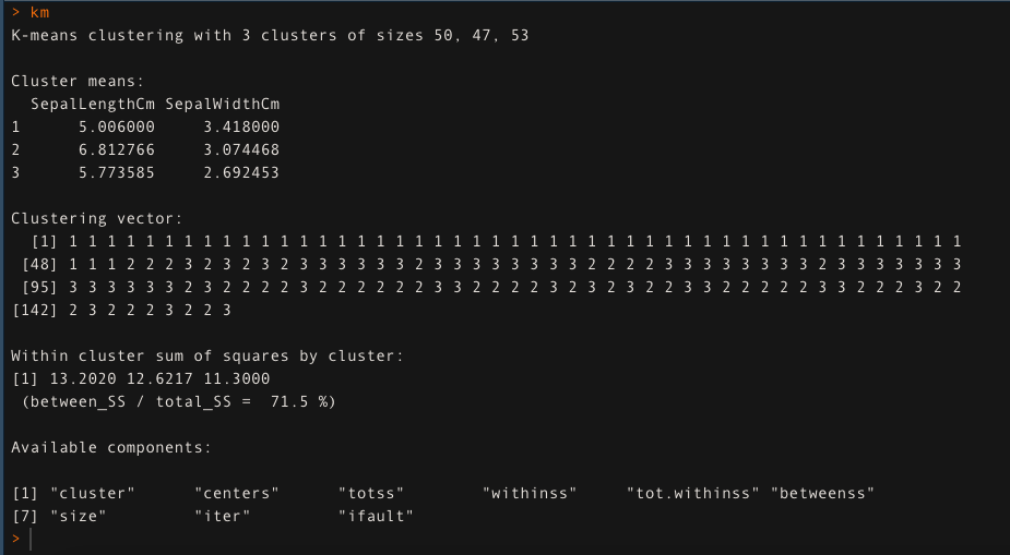
- For k = 3, apply the K-means clustering algorithm. The K-means clustering approach explains the 71,5% of the variability of the data in this case.
km <- kmedias (data[,1:2], k = 3, iter.max = 50)
km
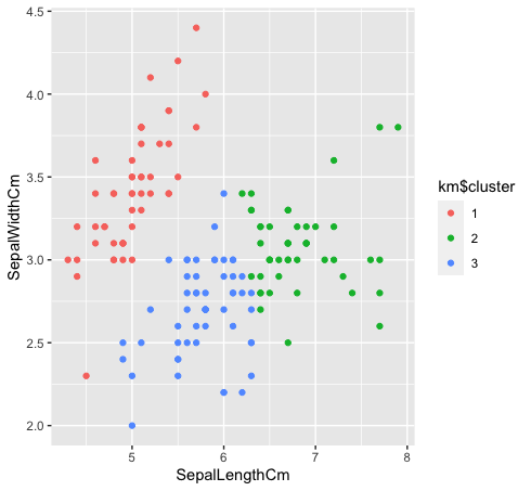
- Let's see how the three classes are grouped by clustering k-means. K-means clustering will not create overlapping clusters, as we all know. Since the species “verde” Y “blue” are not linearly separable in the original data, the grouping of k-means could not capture it because it has reduced groups.
km $ cluster <- as.factor (km $ cluster)
data%>% ggplot (aes (SepalLengthCm, SepalWidthCm, color = km $ cluster)) +
geom_point ()
An article of ~
Shivam Sharma.
The media shown in this article about the K-Means grouping algorithm is not the property of DataPeaker and is used at the author's discretion.


