Descriptive statistics | Descriptive statistical analysis guide

This article was published as part of the Data Science Blogathon.

Introduction

The first step in a data science project is to summarize, describe and visualize the data. Try to know different aspects of the data and its attributes. The best models are created by those who understand their data.

Explore data characteristics and attributes using descriptive statistics. The insights and numerical summary you gain from descriptive statistics help you better understand or be in a position to handle data more efficiently for machine learning tasks.

Descriptive statistics is the default process in data analysis. Exploratory data analysis (EDA) not complete without descriptive statistical analysis.

Then, in this article, I will explain the attributes of the dataset using Descriptive Statistics. It is divided into two parts: Measurement of central data points and Measurement of dispersion. Before starting our analysis, we must complete the data collection and cleaning process.

Data collection and data cleansing

We will collect data from here. I will only use test data for analysis. Puede combinar datos de prueba y de trainingTraining is a systematic process designed to improve skills, physical knowledge or abilities. It is applied in various areas, like sport, Education and professional development. An effective training program includes goal planning, regular practice and evaluation of progress. Adaptation to individual needs and motivation are key factors in achieving successful and sustainable results in any discipline.... for analysis. Here is some code for the data cleaning process of the train data.

Remove from code

• Column Item_Weight and Outlet_Size have null values. These are the options:

1. 1. remove rows containing null values
   2. remove columns containing null values
   3. or replace null values.

• The first 2 options are feasible when data has rows in millions or count of values ​​is small. Then, I will choose the third option to solve the null value problem.
• First, find the Item_Identifier and its corresponding Item_Weight. Then replace what is missing / null in Item_Weight with the known Item_weight of the respective item_identifier.
• As we know, the visibility of items in a store can be close to zero but not zero. Then, We consider 0 as a null value and we follow the previous step for Item_Visibility.
• Outlet_Size is not very important in our analysis and prediction of models. Then, I drop this column.
• Replace LF and reg in Item_fat_content column with Low Fat and Regular Fat.
• Calculate the age of the stores and save these values ​​in the Outlet_years column and drop the Outlet_Establishment_year column.

Let's start with the Descriptive Statistics data analysis.

The measure of the central data point

Finding the numerical and categorical data center using the mean, the medianThe median is a statistical measure that represents the central value of a set of ordered data. To calculate it, the data is organized from lowest to highest and the number in the middle is identified. If there are an even number of observations, the two core values are averaged. This indicator is especially useful in asymmetric distributions, since it is not affected by extreme values.... y la moda se conoce como Medida del punto de datos central. Calculating the center values ​​of the column data by mean, median and mode are different from each other.

Well, then, let's calculate the mean, the median, the count and mode of dataset attributes using python.

1. Tell
   Counting does not directly help find the center of the dataset attributes. But it is used in the calculation of the mean, median and mode. We calculate the total count in each category of the categorical variables. Also calculates the total count of numeric column data.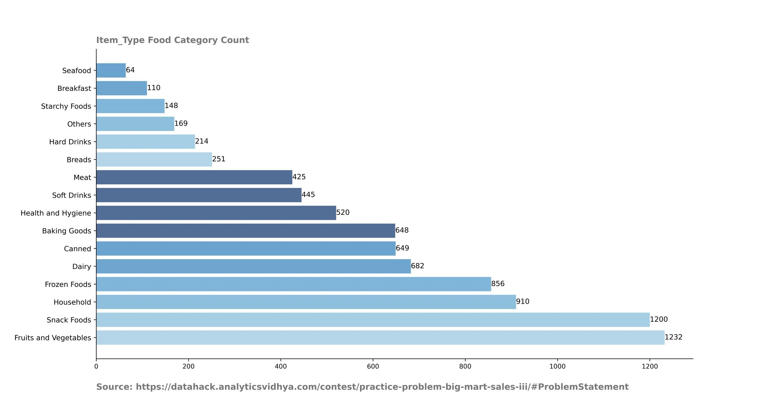

   

   Remove from code.

   • Step through the categorical columns to plot the category and its count.

   Output analysis.

   • These counts help you find out if the data is balanced or not. From this graph, I can say that the ranks of the fruit and vegetable category are much more than the seafood category.
   • We can also assume that sales in the fruit and vegetable category are much more than in the seafood category..

2. To mean

   The sum of the values ​​present in the column divided by the total number of rows in that column is known as the mean. Also known as average.

   Use train.mean () to calculate the mean value of the numeric columns of the train data set.

   Here is some code for categorical columns from the trains dataset.

   print(train[['Item_Outlet_Sales','Outlet_Type']].groupby(['Outlet_Type']).agg({'Item_Outlet_Sales':'mean'}))

   Output analysis

   • The average age of departure is 15 years.
   • Average outlet sales are 2100.
   • The category of supermarket type 3 Outlet_Type's has much more sales than the grocery store category.
   • We can also assume that the supermarket category is more popular than the grocery store category..

3. Median

   The central value of an attribute is known as the median. How do we calculate the median value? First, sort column data in ascending or descending order. Then find the total rows and then divide it by 2.

   That output value is the median of that column.

   The median value divides the data points into two parts. That means the 50% of the data points are present above the median and the 50% under.

   Generally, the median and mean values ​​are different for the same data.

   Median is not affected by outliers. Due to outliers, the difference between the mean and median values ​​increases.

   Use train.median () to calculate the mean value of the numeric columns of the train data set.

   Here is some code for categorical columns from the trains dataset.

   print(train[['Item_Outlet_Sales','Outlet_Type']].groupby(['Outlet_Type']).agg({'Item_Outlet_Sales':'median'}))

   Output analysis

   • Most of the observations are the same as the mean value.
   • The difference in the mean and median value is due to outliers. You can also observe this difference in categorical variables.
4. Way
   The mode is that data point whose count is the maximum in a column. There is only one mean and median value for each column. But attributes can have more than one mode value. Use train.mode () to calculate the mean value of the numeric columns of the train data set. Here is some code for the categorical columns of the train dataset.

   print(train[['Item_Outlet_Sales',
   'Outlet_Type',
   'Outlet_Identifier',
   'Item_Identifier']].groupby(['Outlet_Type']).agg(lambda x:x.value_counts().index[0]))

   Output analysis

   • Outlet_Type has a mode value. Supermarket type 1. The supermarket type category 1 best selling item or mode value is FDZ15.
   • Item_Identifier FDH50 is the best-selling item among the Outlet_Type category.

Measures of dispersion

A measure of dispersion explains how diverse the attribute values ​​are in the data set. Also known as a measure of spread. From this statistic, get to know how and why data is propagated from one point to another.

These are the statistics that go into the dispersion measure.

• Distance
• Percentiles or quartiles
• Standard deviation
• Difference
• Obliquity

1. Distance

   The difference between the maximum value and the minimum value in a column is known as the range.

   Here is a code to calculate the range.

   for i in num_col:
       print(f"Column: {i} Max_Value: {max(train[i])} Min_Value: {min(train[i])} Range: {round(max(train[i]) - min(train[i]),2)}")

   You can also calculate the rank of categorical columns. Here is a code to find out the minimum and maximum values ​​in each output category.

   Output analysis

   • The range of Item_MRP and Item_Outlet_sales is high and may need transformation.
   • There is a great variation in Item_MRP in the category of supermarket type 3.
2. Percentiles or quartilesWe can describe the distribution of the column values ​​by calculating the summary of several percentiles. The median is also known as the percentile 50 of the data. Here is a different percentile.
   • The minimum value is equal to the percentile 0.
   • The maximum value equals the percentile 100.
   • The first quartile equals the percentile 25.
   • The third quartile equals the percentile 75.

   Here is a code to calculate the quartiles.

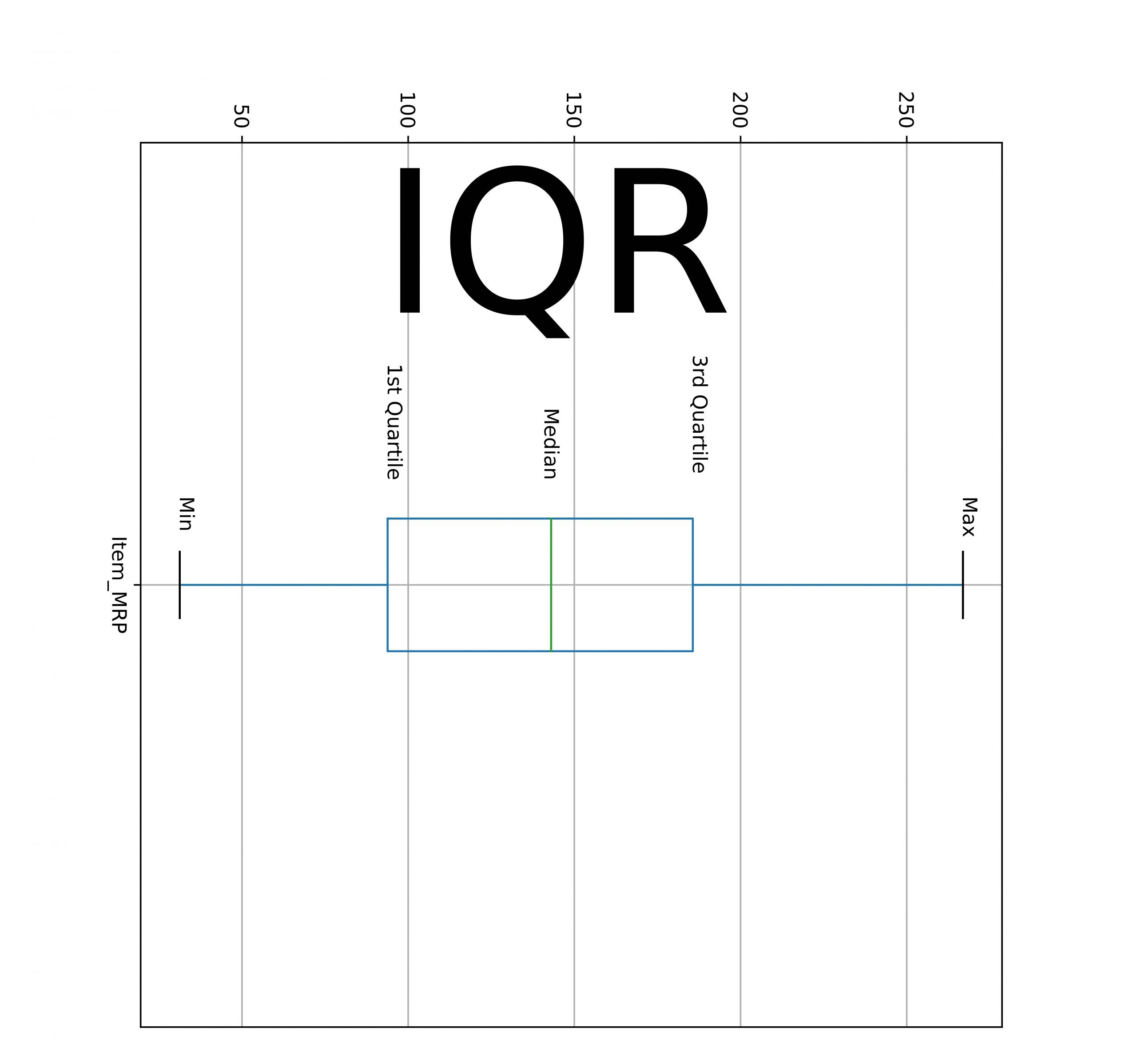
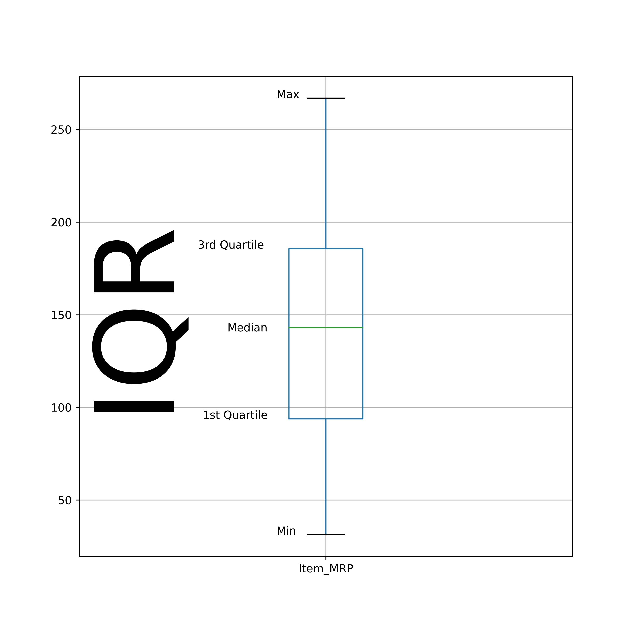
   The difference between 3rd and the 1S t The quartile is also known as the interquartile (IQR). What's more, maximum data points are included in IQR.

   

3. Standard deviation

   The value of the standard deviation tells us how much all the data points deviate from the mean value. The standard deviation is affected by outliers because it uses the mean for its calculation.

   Here is a code to calculate the standard deviation.

   for i in num_col:
       print(i , round(train[i].std(),2))

   Pandas also have a shortcut to calculate all the above statistic values.

   Train.describe()

4. DifferenceThe variance is the square of the standard deviation. In the case of outliers, the value of the variance becomes large and noticeable. Therefore, is also affected by outliers. Here is a code to calculate the variance

   for i in num_col:
       print(i , round(train[i].where(),2))

   Output analysis.

   • Item_MRP and Item_Outlet_sales columns have a large variance due to outliers.

5. Obliquity

   Ideally, the data distribution should be in Gaussian form (bell curve). But practically, data shapes are skewed or skewed. This is known as skew in the data..

   You can calculate the skewness of the train data using train.skew (). The bias value can be negative (left) the positive (right). Its value must be close to zero.

Final notes

These are the statistics we turn to when conducting exploratory data analysis on the dataset. You should pay attention to the values ​​generated by these statistics and ask why this number. These statistics help us determine the attributes for data transformation and removal of variables from post-processing..

The Pandas library has really good functions that help you get descriptive statistics values ​​in one line of code.

Related