Introduction
Exploratory data analysis is one of the best practices used in data science today. When starting a career in data science, people generally don't know the difference between data analysis and exploratory data analysis. There is not a big difference between the two, but they both have different purposes.

Exploratory data analysis (EDA): exploratory data analysis is a complement Inferential statistics, which tends to be quite rigid with rules and formulas. At an advanced level, EDA involves looking at and describing the data set from different angles and then summarizing it.
Analysis of data: data analysis is the statistics and probability of discovering trends in the data set. Used to display historical data by using some analysis tools. Helps break down information to transform metrics, facts and figures on improvement initiatives.
Exploratory data analysis (EDA)
We will explore a dataset and perform exploratory data analysis in Python. You can check our python course online to get on board with Python.
The main topics to be covered are as follows:
– Handle missing value
– Remove duplicates
– Treatment of outliers
– Normalization and scaling (numeric variables)
– Coding of categorical variables (dummy variables)
– Bivariate analysis
# Libraries import
# Loading the dataset
We will load the Excel file of EDA cars using pandas. For this, we will use the read_excel file.
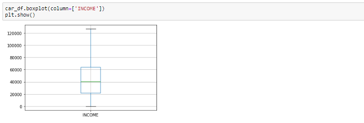
Box plot after removing outliers
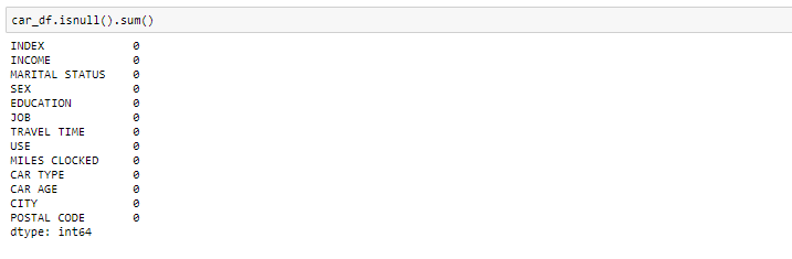
# Basic data exploration
In this step, we will perform the following operations to verify what the data set is made of. We will check the following things:
– dataset manager
– the shape of the data set
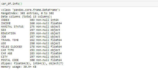
– dataset information
– dataset summary
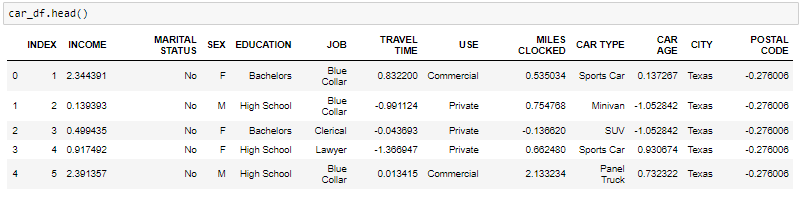
- The head function will tell you the best records in the dataset. By default, Python shows you only the 5 main registers.
-
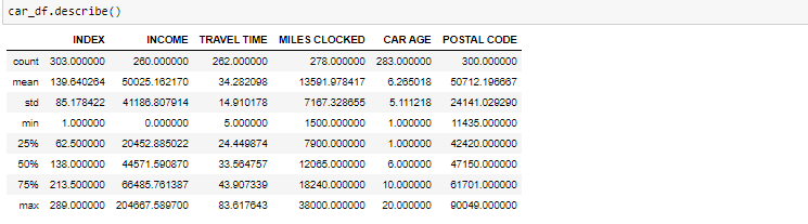
The shape attribute tells us a series of observations and variables that we have in the data set. It is used to verify the dimension of the data. The automobile dataset has 303 observations and 13 variables in the data set.

-
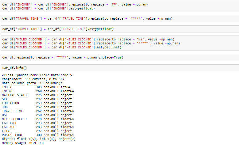
info () used to verify information about data and data types of each respective attribute.

By looking at the data in the main function and in the information, we know that the variable Revenue and the travel time are of the floating data type instead of the object. Then we'll make it the float. What's more, there are some invalid values like @@ and ‘*'In the data that we will treat as missing values.

-
The described method will help to see how the data has been distributed for numerical values. We can clearly see the minimum value, mean values, different percentile values and maximum values.


Handling missing value
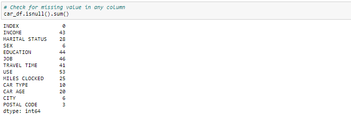
We can see that we have several missing values in the respective columns. There are several ways to deal with missing values in the dataset. And what technique to use when it really depends on the type of data you are dealing with.
- Eliminate missing values: in this case, we eliminate the missing values of those variables. In case of very few missing values, can delete them.
- Impute with mean value: for the numeric column, you can replace missing values with mean values. Before replacing with the mean value, it is advisable to verify that the variable should not have extreme values .ie outliers.
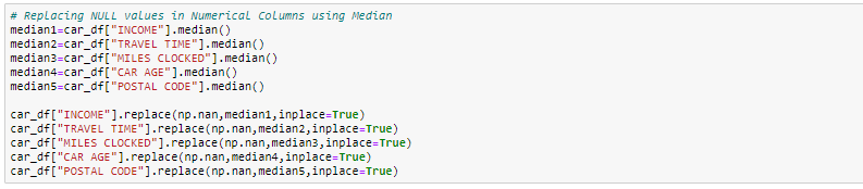
- Impute with median value: for the numeric column, you can also replace missing values with median values. In case you have extreme values, as outliers, it is advisable to use the median method.
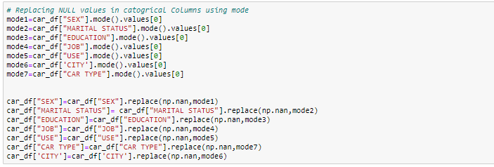
- Impute with mode value: for the categorical column, you can replace missing values with mode values, namely, the frequent.
In this exercise, we will replace the numeric columns with median values and, for categorical columns, we will delete the missing values.
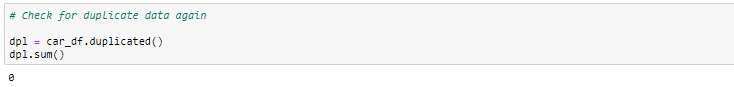
Handling duplicate records
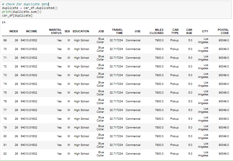
Since we have 14 duplicate records in the data, we will remove it from the dataset to get only distinct records. After removing the duplicate, we will check if the duplicates have been removed from the dataset or not.
![]()
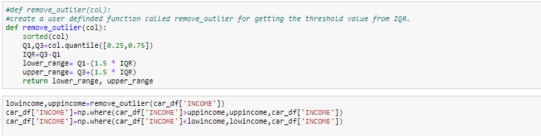
Handling of outliers
Outliers, being the most extreme observations, can include the maximum or minimum of the sample, the both, depending on whether they are extremely high or low. But nevertheless, the sample maximum and minimum are not always outliers because they may not be unusually far from other observations.
We usually identify outliers with the help of the box plot, so here the boxplot shows some of the data points outside the data range.
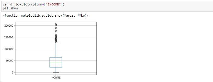
Box plot before removing outliers
Looking at the box plot, it seems that the variables INCOME, have outliers present in the variables. These outliers need to be taken into account and there are several ways to deal with them:
- Remove the outlier
- Replace the outlier using the IQR
#Boxplot After removing the outlier
Bivariate analysis
When we talk about bivariate analysis, means analyze 2 variables. As we know that there are numerical and categorical variables, there is a way to parse these variables as shown below:
-
Numeric vs numeric
1. Dispersion diagram
2. Line graph
3. Heat map for correlation
4. Joint plot -
Categorical vs Numerical
1. Bar graphic
2. Violin frame
3. Categorical box plot
4.warm plot -
Two categorical variables
1. Bar graphic
2. Clustered bar chart
3. Dot chart
If we need to find the correlation-
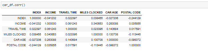
Correlation between all variables
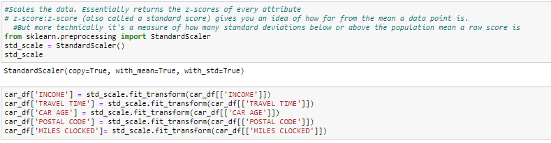
Normalize and scale
Often, the variables in the data set are of different scales, namely, one variable is in millions and others in only 100. For instance, in our dataset, income has values in thousands and age in just two digits. Since the data of these variables are of different scales, it is difficult to compare these variables.
The scale of characteristics (also known as data normalization) is the method used to standardize the range of characteristics of the data. Since the range of data values can vary widely, becomes a necessary step in data preprocessing while using machine learning algorithms.
In this method, we convert variables with different measurement scales into a single scale. StandardScaler normalizes the data using the formula (x-mean) / standard deviation. We will do this only for numeric variables.
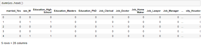
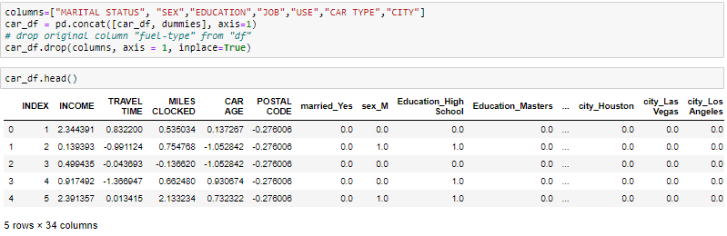
CODING
One-Hot-Encoding is used to create dummy variables to replace the categories in a categorical variable in characteristics of each category and represent it using 1 O 0 according to the presence or absence of the categorical value in the registry.
This is necessary, since machine learning algorithms only work with numeric data. That is why it is necessary to convert the categorical column into numeric.
get_dummies is the method that creates a dummy variable for each categorical variable.

About the Author

Ritika Singh | – Data scientist
I am a data scientist by profession and a blogger by passion. I have worked on machine learning projects for over 2 years. Here you will find articles on “Machine Learning, Stats, Deep Learning, NLP and Artificial Intelligence".


