Analysis of employee attrition using logistic regression with R

This article was published as part of the Data Science Blogathon.

“To win in the market, you must win in the workplace” –Steve Jobs, founder of Apple Inc..

Introduction

Why do we use logistic regression to analyze employee attrition?

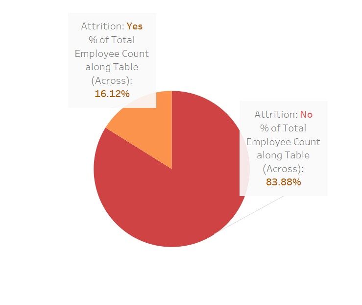
If an employee is going to stay or leave a company, your answer is simply binomial, namely, could be “YES” O “NO”. Then, we can see that our dependent variable Employee Attrition is just a categorical variable. In the case of a categorical dependent variable, we can't use linear regression, then, We have to use "LOGISTIC REGRESSION“.

Methodology

Here, I am going to wear 5 Simple steps to analyze employee attrition using R software

1. DATA COLLECTION
2. DATA PRE-PROCESSING
3. DIVIDING THE DATA INTO TWO PARTS “TRAINING” Y “TESTS”
4. BUILD THE MODEL WITH “TRAINING DATA SET”
5. DO THE PRECISION TEST USING THE “TEST DATA SET”

Data exploration

This data set is collected from the IBM Human Resources department. The data set contains 1470 observations and 35 variables. Within 35 variables, "Wear" is the dependent variable.

A quick look at the dataset:

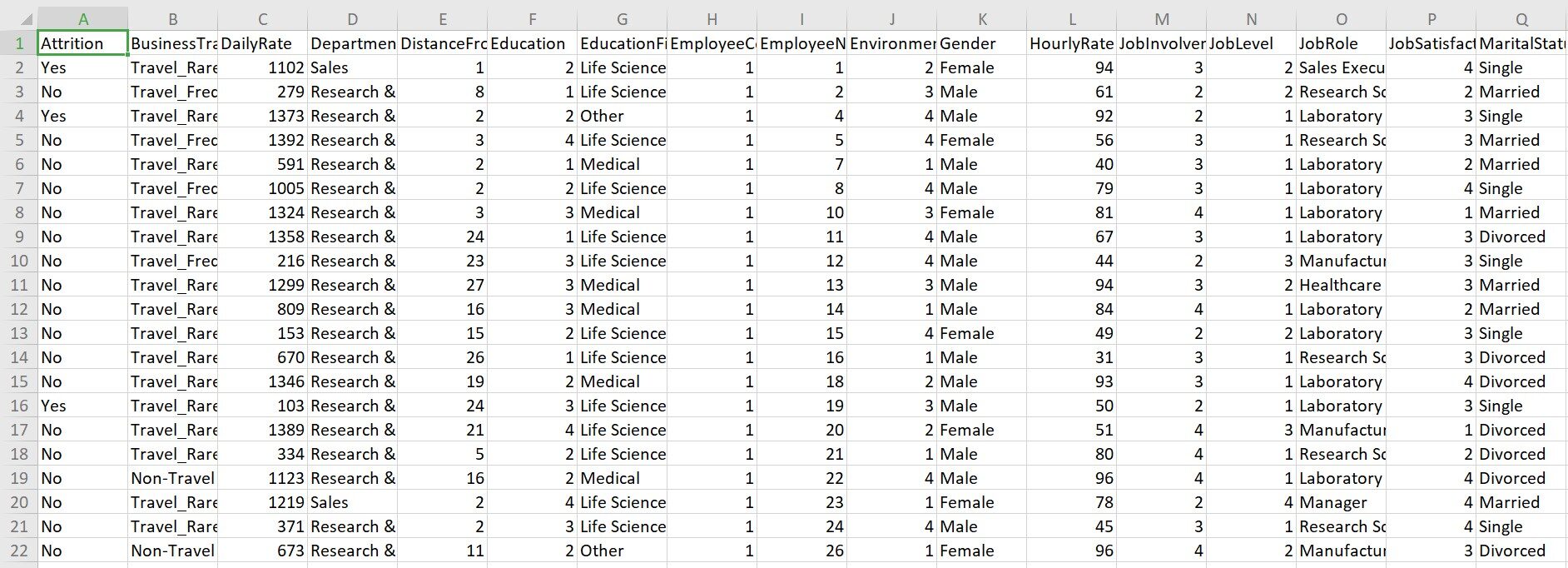
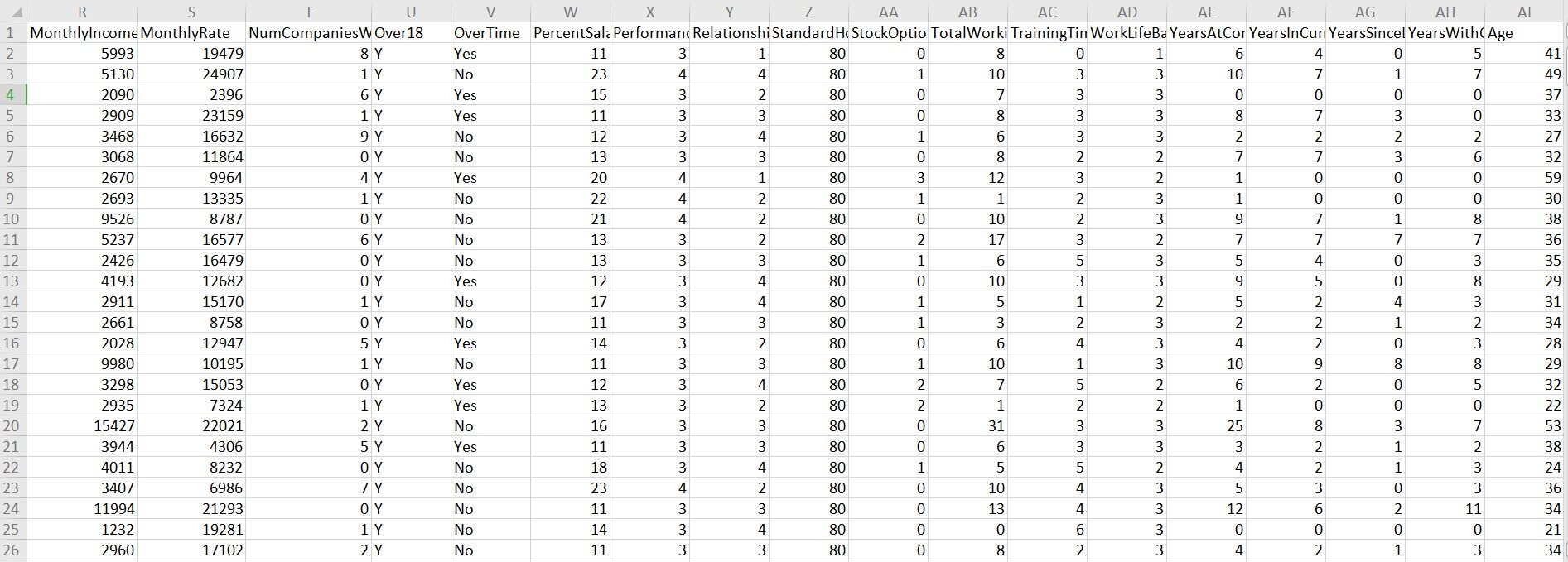
Have a look:

Data preparation

• Change data types:

  First, we have to change the data type of the dependent variable “Wear”. It is given in the form of "Yes" and "No", namely, is a categorical variable. To make a suitable model we have to convert it into numerical form. For it, we will assign the value 1 to "Yes" and the value 0 to "No" and we will convert it to numeric.

  JOB_Attrition$Attrition[JOB_Attrition$Attrition=="Yes"]=1
  JOB_Attrition$Attrition[JOB_Attrition$Attrition=="No"]=0
  JOB_Attrition$Attrition=as.numeric(JOB_Attrition$Attrition)

  next, we will change all the variables from “character” a “Factor”

  There is 8 character variables: business trip, Department, education, educational field, gender, job function, marital status, over time. The column numbers are 2, 4, 6, 7, 11, 15, 17, 22 respectively.

  JOB_Attrition[,c(2,4,6,7,11,15,17,22)]=lapply(JOB_Attrition[,c(2,4,6,7,11,15,17,22)],as.factor)

  Finally, there is another variable “Over 18” which has all the inputs like “Y”. It is also a character variable. We will transform into numerical since it only has one level so transforming into factor will not give a good result. For it, we will assign the value 1 to "Y" and we will transform it into numeric.

  JOB_Attrition$Over18[JOB_Attrition$Over18=="Y"]=1
  JOB_Attrition$Over18=as.numeric(JOB_Attrition$Over18)

Divide the data set into “training” Y “proof”

In any regression analysis, we have to divide the data set into 2 parts:

1. TRAINING DATA SET
2. TEST DATA SET

With the help of the training dataset, we will create our model and test its accuracy using the test data set.

set.seed(1000)
ranuni=sample(x=c("Training","Testing"),size=nrow(JOB_Attrition),replace=T,prob=c(0.7,0.3))
TrainingData=JOB_Attrition[ranuni =="Training",]
TestingData=JOB_Attrition[ranuni =="Testing",]
nrow(TrainingData)
nrow(TestingData)

We have successfully divided the entire dataset into two parts. Now we have 1025 Training data and 445 Test data.

Building the model

Now we are going to build the model following a few simple steps as follows:

1. Identify the independent variables
2. Incorporate the dependent variable “Wear” in the model.
3. Transform the data type of the model “character” a “formula”
4. Incorporate TRAINING data into the formula and build the model

independentvariables = colnames(JOB_Attrition[,2:35])
independentvariables
Model=paste(independentvariables,collapse="+")
Model
Model_1=paste("Attrition~",Model)
Model_1
class(Model_1)
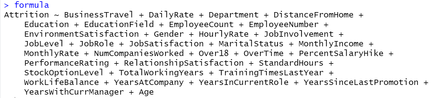
formula=as.formula(Model_1)
formula

Production:

Next, We will incorporate "Training data" into the formula using the "glm" function and build a logistic regression model..

Trainingmodel1=glm(formula = formula,data=TrainingData,family="binomial")

Now, we are going to design the model by the “Step-by-step selection”Method to obtain significant variables from the model. Executing the code will give us an output list where variables are added and removed based on our importance of the model. The AIC value at each level reflects the goodness of the respective model. As the value keeps falling, a logistic regression model is obtained that fits better.

The application of the summary on the final model will give us the list of final significant variables and their respective important information..

Trainingmodel1=step(object = Trainingmodel1,direction = "both")
summary(Trainingmodel1)

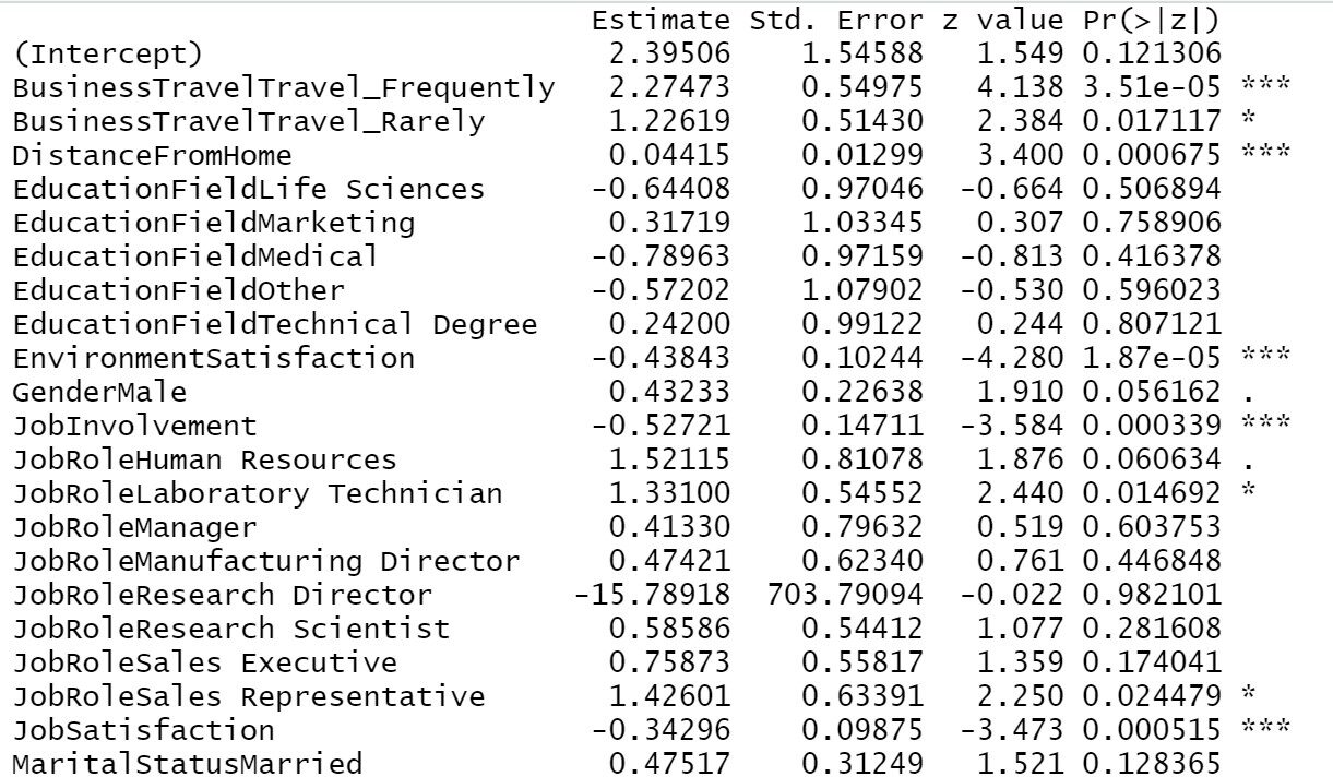
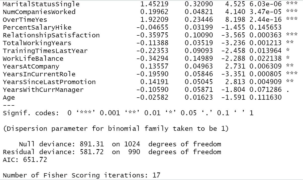
From our previous result we can see, Business trip, Distance from home, Satisfaction with the environment, Labor involvement, Work satisfaction, Marital status, Number of companies worked, Over time, Satisfaction in relationships, Total working years, Years in the company, years since the last promotion, years in current position all of these are the most important variables in determining employee attrition. If the company deals mainly with these areas, there will be less chance of losing an employee.

A quick visualization to see how much these variables affect the “wear”

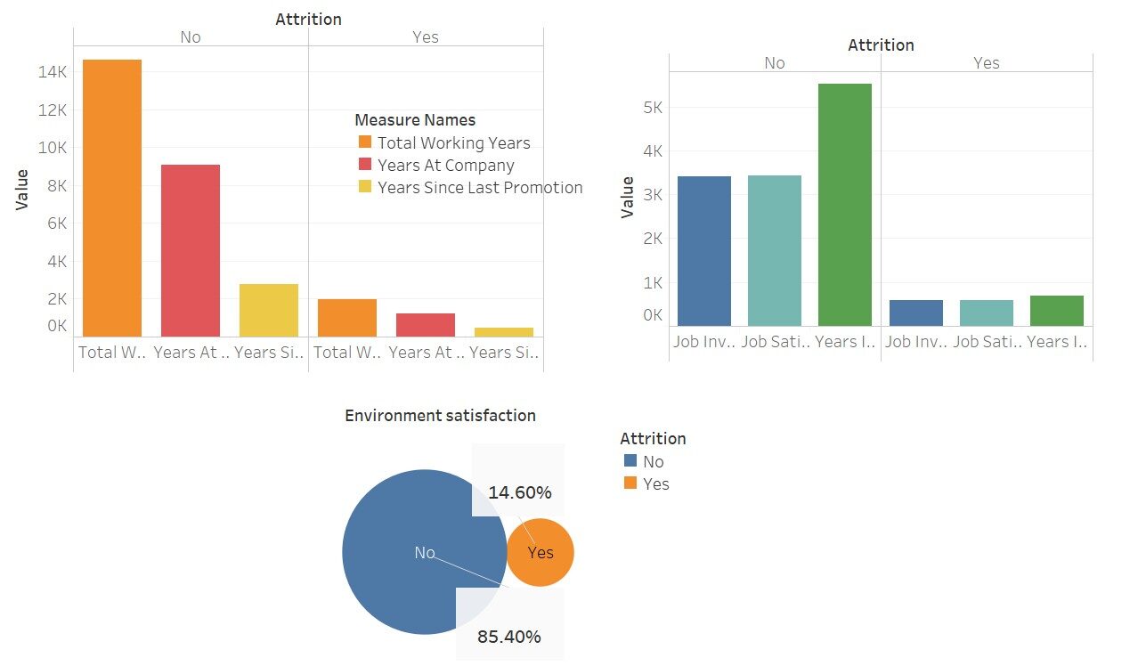
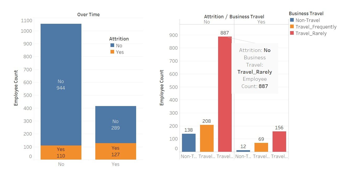
Here I have used Tableau for these visualizations; not beautiful This software just makes our job easier.

Now, we can realize the Hoshmer-Lemes show goodness-of-fit test on the data set, to judge the precision of the predicted probability of the model.

The hypothesis is:

H0: The model fits well.

H1: The model does not fit well.

And, p value> 0,05 we will accept H0 and reject H1.

To perform the test in R we need to install the mkMisc package.

HLgof.test(fit=Trainingmodel1$fitted.values,obs=Trainingmodel1$y)

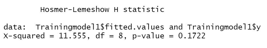
Here, we can see that the p-value is greater than 0.05, therefore we will accept H0. Now, it is proven that our model is well adjusted.

Generating a ROC Curve for Training Data

Another technique to analyze the goodness of fit of the logistic regression is the ROC measures (receiver operating characteristics). ROC measures are sensitivity, specificity 1, false positive and false negative. The two measures we use widely are sensitivity and specificity.. Sensitivity measures the goodness of the model's accuracy, while the specificity measures the weakness of the model.

To do this in R we need to install a package pROC.

barter = rock(response=Trainingmodel1$y,predictor = Trainingmodel1$fitted.values,plot=T)
barter $ auc

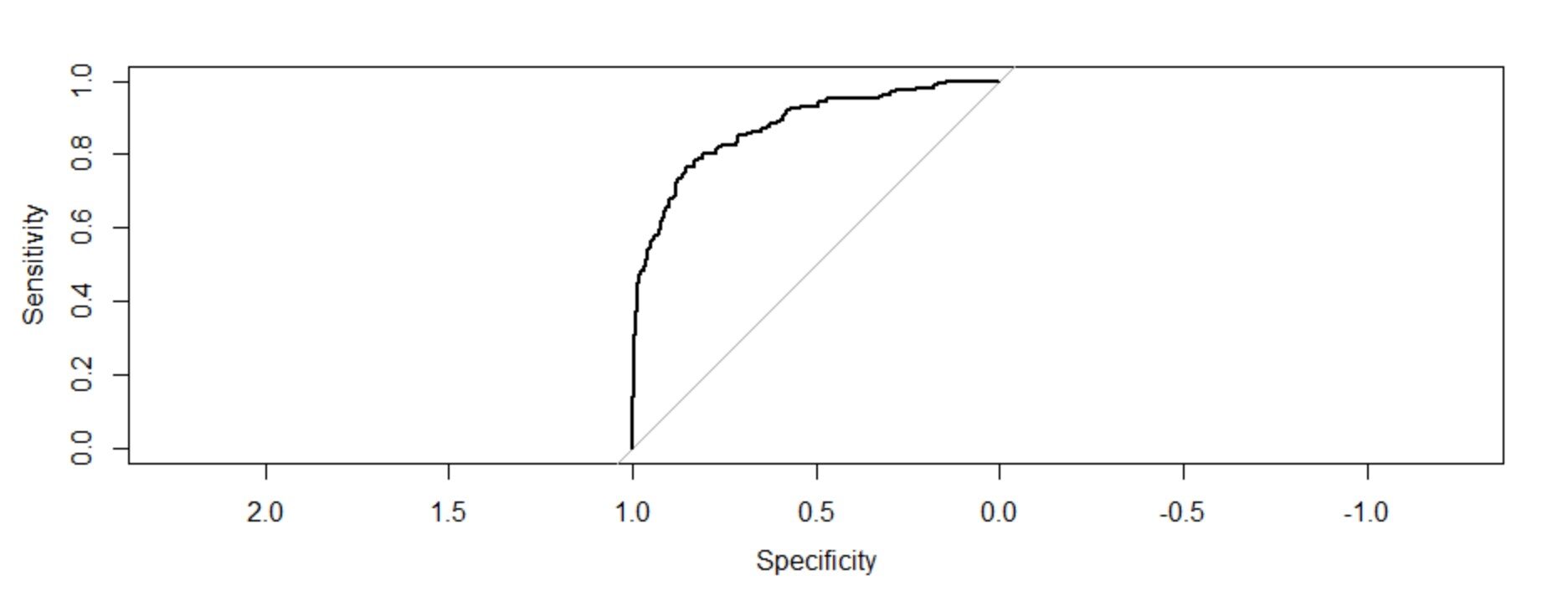
The area under the curve: 0.8759

Interpretation of the figure:

The graph of these two measurements gives us a concave graph that shows how the sensitivity is increasing 1-the specificity is increasing but at a decreasing rate. The C value (AUC) o the value of the concordance index gives the measure of the area under the ROC curve. If c = 0,5, would have meant that the model cannot perfectly discriminate between 0 Y 1 answers. It then implies that the initial model cannot perfectly say which employees are going to leave and who are going to stay..

But here we can see that our value c is much greater than 0.5. It is 0,8759. Our model can perfectly discriminate between 0 Y 1. Therefore, we can successfully conclude that it is a well-adjusted model.

Creating the leaderboard for the training dataset:

trpred=ifelse(test=Trainingmodel1$fitted.values>0.5,yes = 1,no=0)
table(Trainingmodel1$y,trpred)

The above code sets, the predicted value of the probability greater than 0, .5, then the value of the state is 1, otherwise it is 0. based on this criterion, this code re-labels the answers “Yes” Y “No” of “Wear”. Now, it is important to understand the percentage of predictions that match the initial belief obtained from the data set. Here we will compare the pair (1-1) Y (0-0).

Have 1025 training data. We have predicted {(839 + 78) / 1025} * 100 =89% correctly.

Comparing the result with the test data:

Now we will compare the model with the test data. It is a lot like a precision test.

testpred=predict.glm(object=Trainingmodel1,newdata=TestingData,type = "response")
testpred
tsroc=roc(response=TestingData$Attrition,predictor = testpred,plot=T)
tsroc $ auc

Now, we have incorporated test data into the training model and we will see the ROC.

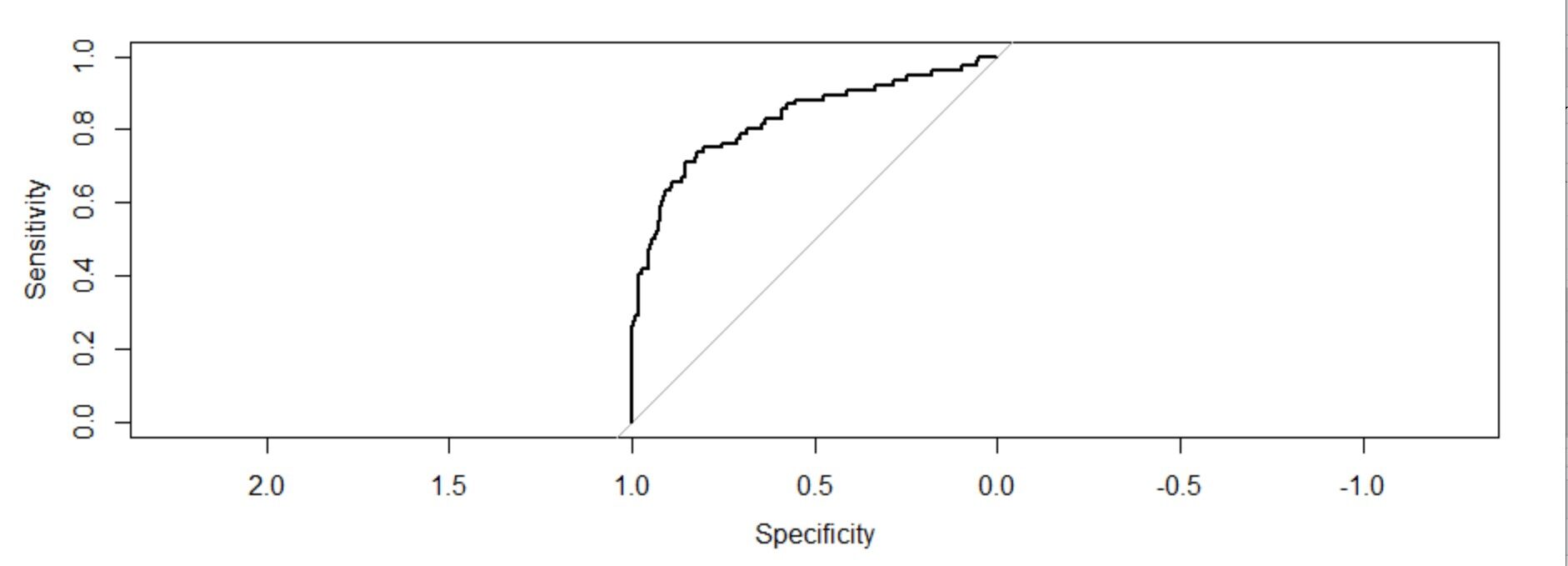
The area under the curve: 0,8286 (c value). It is also far superior to 0,5. It is also a well fitted model.

Create the classification table for the test dataset

testpred = ifelse(test = testpred>0.5,yes=1,no=0)
table(TestingData$Attrition,testpred)

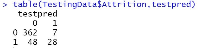
Have 445 test data. we have correctly predicted {(362 + 28) / 445} * 100 =87,64%.

Due, we can say that our logistic regression model is a very well fitted model. Any set of employee attrition data can be analyzed using this model.

What do you think is a good model? Comment below

CONCLUSION:

We have successfully learned how to analyze employee attrition using "LOGISTIC REGRESSION" with the help of R software. Just with a couple of codes and a proper data set, a company can easily understand which areas they need to take care of in order to make the workplace more comfortable for their employees and restore the energy of their human resources for a longer period.

Featured image is taken from trainingjournal.com

Link to my LinkedIn profile:

https://www.linkedin.com/in/tiasa-patra-37287b1b4/

Related