This article was published as part of the Data Science Blogathon
Creating facial recognition is considered a very easy task in the field of computer vision., but it is extremely difficult to have a pipeline that can predict faces with complex backgrounds when you have multiple faces, different lighting conditions and different image scales. This blog will describe how we create a model that can outperform humans in some cases. Our dataset consists of 3 lessons (I cannot share the data due to confidentiality issues, but i'll show you how it looks). Class 1 it Jesse Eisenberg (actor), class 2 is Mila Kunis (pop star) and the class 0, Anyone. This is what our train looked like (80 images) and test data (more of 1800 images).
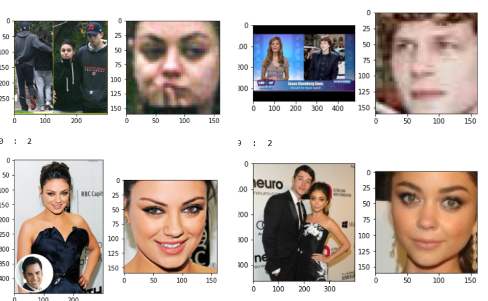
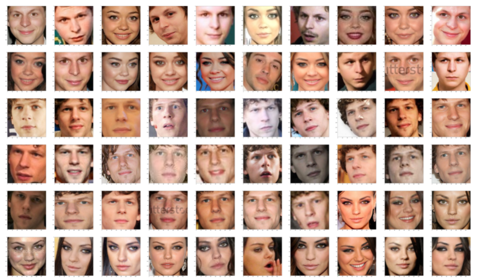
These are our test data and the faces extracted from those images, this data is extremely complex due to multiple faces, complex backgrounds and lots of pixelated images. Secondly, our train data is extremely clean as shown in the picture below. We have many differences in the distribution of test and train data. We need a technique that can generalize well regardless of how many samples you need and how different the train and test data are.
The technique that we are going to use for this task is, first, generate the facial key from a deep learning model and then apply a simple classifier.
Using FACENET
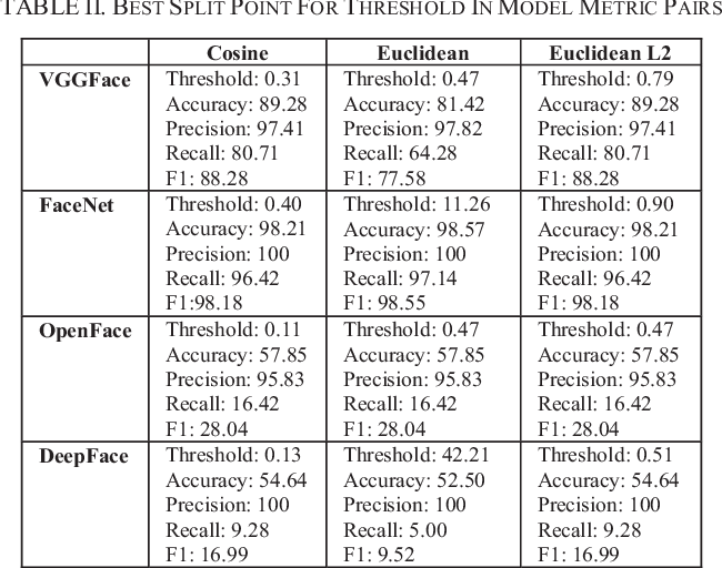
To really push the limits of face detection, we will see some cutting edge methods. Modern face extraction techniques have made use of Deep Convolution Networks. As we all know, the features created by modern deep learning frameworks are actually better than most hand-built features. We check 4 deep learning models, namely, FaceNet (Google), DeepFace (Facebook), VGGFace (Oxford) and OpenFace (CMU). Of these 4 Models FaceNet it was giving us the best result. In general, FaceNet offers better results than the others 3 Models.
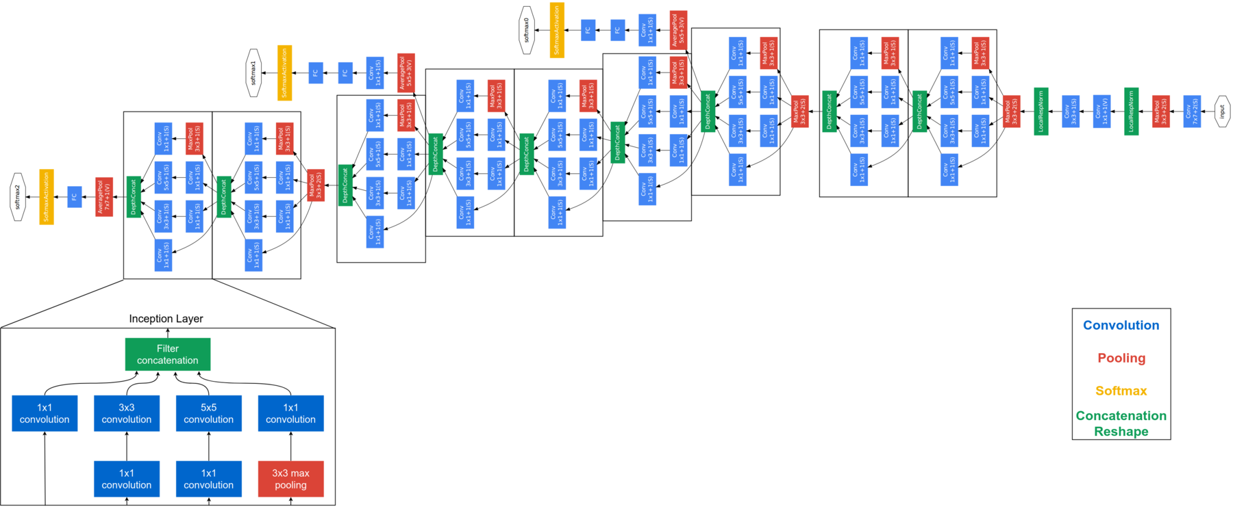
FaceNet is considered a next-generation model developed by Google. It is based on the initial layer, explaining the full architecture of FaceNet is beyond the scope of this blog. The architecture of FaceNet is shown below. FaceNet uses block start modules to reduce the number of trainable parameters. This model takes RGB images of 160 × 160 and generates an embed of size 128 for a picture. For this implementation, we will need a couple of additional functions. But before sending the face image to FaceNet, we need to extract the faces from the images.
detector = dlib.cnn_face_detection_model_v1("../input/pretrained-models-faces/mmod_human_face_detector.dat")

def rect_to_bb(rect):
    # take a bounding predicted by dlib and convert it
    # to the format (x, Y, w, h) as we would normally do
    # with OpenCV
    x = rect.rect.left()
    y = rect.rect.top()
    w = rect.rect.right() - x
    h = rect.rect.bottom() - Y

    # return a tuple of (x, Y, w, h)
    return (x, Y, w, h)

def dlib_corrected(data, data_type="train"):
    #We set the size of the image
    dim = (160, 160)
    data_images=[]
    #If we are processing training data we need to keep track of the labels
    if data_type=='train':
        data_labels=[]
    #Loop over all images
    for cnt in range(0,len(data)):
        image = data['img'][cnt]
        #The large images are resized
        if image.shape[0] > 1000 and image.shape[1] > 1000:
            image = cv2.resize(image, (1000,1000), interpolation = cv2.INTER_AREA)
        #The image is converted to grey-scales
        gray = cv2.cvtColor(image, cv2.COLOR_BGR2GRAY)
        #Detect the faces
        rects = detector(gray, 1)
        sub_images_data = []
        #Loop over all faces in the image
        for (i, rect) in enumerate(rects):
            #Convert the bounding box to edges
            (x, Y, w, h) = rect_to_bb(rect)
            #Here we copy and crop the face out of the image
            clone = image.copy()
            if(x>=0 and y>=0 and w>=0 and h>=0):
                crop_img = clone[Y:y+h, x:x+w]
            else:
                crop_img = clone.copy()
            #We resize the face to the correct size
            rgbImg = cv2.resize(crop_img, dim, interpolation = cv2.INTER_AREA)
            #In the test set we keep track of all faces in an image
            if data_type == 'train':
                sub_images_data = rgbImg.copy()
            else:
                sub_images_data.append(rgbImg)
        #If no face is detected in the image we will add a NaN
        if(len(rects)==0):
            if data_type == 'train':
                sub_images_data = np.empty(dim + (3,))
                sub_images_data[:] = np.nan
            if data_type=='test':
                nan_images_data = np.empty(dim + (3,))
                nan_images_data[:] = np.nan
                sub_images_data.append(nan_images_data)
        #Here we add the the image(s) to the list we will return
        data_images.append(sub_images_data)
        #And add the label to the list
        if data_type=='train':
            data_labels.append(data['class'][cnt])
    #Lastly we need to return the correct number of arrays
    if data_type=='train':
        return np.array(data_images), np.array(data_labels)
    else:
        return np.array(data_images)
USANDO DLIB
DLIB is a widely used model for detecting faces. In our experiments, we found that dlib produces better results than HAAR, although we note that some improvements can still be made:
- If the boundaries of the rectangle face are moved out of the image, we take the whole image instead of the face cutout. It is implemented as follows:
- and (x> = 0 and and> = 0 y w> = 0 y h> = 0):
- crop_img = clon[Y:y+h, x:x+w]
- the rest:
- and (x> = 0 and and> = 0 y w> = 0 y h> = 0):
- For test images, instead of saving one face per image, we save all faces for prediction.
- Instead of a HOG-based detector, we can use a detector based on CNN. How these enhancements are designed to optimize your use with FaceNet, we will define a new corrected face detection.
The above code block extracts the faces from the image, for many images we have several faces, so we must put all those faces in a list. To extract the faces we are using dlib.cnn_face_detection_model_v1, note that you should not feed very large dimension images to this, otherwise you will get a dlib memory error. If an image does not have a face, stores NaN in those places. Let's FaceNet these data images now. The above pre-processing is only required for test data, the train data is already clean, what can be seen in the pictures above. Once we are done getting the face inlays from the train data, get face inlays for test data, but first you have to use the preprocessing provided in the code block above to extract faces from the test data.
def get_embedding(model, face_pixels):
    # scale pixel values
    face_pixels = face_pixels.astype('float32')
    # standardize pixel values across channels (global)
    mean, std = face_pixels.mean(), face_pixels.std()
    face_pixels = (face_pixels - mean) / std
    # transform face into one sample
    samples = expand_dims(face_pixels, axis=0)
    # make prediction to get embedding
    yhat = model.predict(samples)
    return yhat[0]

model = load_model('../input/pretrained-models-faces/facenet_keras.h5')

svmtrainX = []
for index, face_pixels in enumerate(newTrainX):
    embedding = get_embedding(model, face_pixels)
    svmtrainX.append(embedding)
After generating the inlays for training and testing, we will use SVM for classification. Why SVM, You can ask? With much experience, I have come to know that SVM-based functions + DL can outperform any other method, even to deep learning methods, when the amount of data is small.
from sklearn.svm import SVC
from sklearn.pipeline import make_pipeline
from sklearn.naive_bayes import GaussianNB
from sklearn.neural_network import MLPClassifier
from sklearn.preprocessing import StandardScaler, MinMaxScaler, Normalizer

linear_model = make_pipeline(StandardScaler(), SVC(kernel="rbf", C=1.0, gamma=0.01, probability =True))
linear_model.fit(svmtrainX, svmtrainY)
Once the SVM is trained, time to do some tests, but our test data has multiple faces in a list. Then, as long as we have Jesse or Mila in a picture, we will ignore the class 0 and when both Jesse and Mila are present in a picture, then we will choose the one that gives us the greatest precision.
predicitons=[]
for i in corrected_test_X:
    flag=0
    if(len(i)==1):
        embedding = get_embedding(model, i[0])
        tmp_output = linear_model.predict([embedding])
        predicitons.append(tmp_output[0])
    else:
        tmp_sub_pred = []
        tmp_sub_prob = []
        for j in i:
            j= j.astype(int)
            embedding = get_embedding(model, j)
            tmp_output = linear_model.predict([embedding])
            tmp_sub_pred.append(tmp_output[0])
            tmp_output_prob = linear_model.predict_log_proba([embedding])
            tmp_sub_prob.append(np.max(tmp_output_prob[0]))

        if 1 in tmp_sub_pred and 2 in tmp_sub_pred:
            index_1 = np.where(np.array(tmp_sub_pred)==1)[0][0]
            index_2 = np.where(np.array(tmp_sub_pred)==2)[0][0]
            if(tmp_sub_prob[index_1] > tmp_sub_prob[index_2] ):
                predicitons.append(1)
            else:
                predicitons.append(2)
        elif 1 not in tmp_sub_pred and 2 not in tmp_sub_pred:
            predicitons.append(0)
        elif 1 in tmp_sub_pred and 2 not in tmp_sub_pred:
            predicitons.append(1)
        elif 1 not in tmp_sub_pred and 2 in tmp_sub_pred:
            predicitons.append(2)
DISCUSSION
Final remarks, this is a very small data set, so the results can change enormously even when adding or removing some images. In our test we found out that he cheated on us many times, there was around 20 images in the test that were incorrectly predicted by us but correctly predicted by our model. We confirm the expected result by searching those images on Google.
Deep neural networks can extract more meaningful features than machine learning models. But nevertheless, the downfall of these large networks is the need for a large amount of data. We managed to deal with this problem using a previously trained model, a model that has been trained on a much larger data set to retain knowledge of how to encode facial images, which we then use for our purposes in this challenge. What's more, SVM's fine tuning really helped us go beyond the precision of the 95%.


