Image and text similarity | Introduction to the similarity of images and text

Introduction

Image analysis and mapping in Earth Engine using NDVI ", now is another article on image analysis again. Unlike the previous article, this article analyzes general image analysis, no Satellite image analysis. The objective of this discussion is to detect whether two products are the same or not.. Each of the two products has image and text names. If the product pair has similar or the same images or text names, that means the two products are the same. The data comes from a competition held at Kaggle.

There is 4 basic packages used in this script: NumPy, pandas, matplotlib y seaborn. There are also other specific packages. “Image” load and display image data. “Imagehash” calculates the similarity of two images. “Fuzzywuzzy” detects the similarity of two texts. The “metrics” The package calculates the accuracy score of the true label and the predicted label.

# import packages
import numpy as np
import pandas as pd
import matplotlib.pyplot as plt
import seaborn as sns
from PIL import Image
import imagehash
from fuzzywuzzy import fuzz
from sklearn.tree import DecisionTreeClassifier
from sklearn import metrics

Image similarity

The similarity of the two images is detected by the package “imagehash”. If two images are identical or almost identical, the image hash difference will be 0. Two images are more similar if the image hash difference is closer to 0.

Comparing the similarity of two images with imagehash consists of 5 Steps. (1) Images are converted to grayscale. (2) Image sizes are reduced to be smaller, for instance, a 8 × 8 pixels by default. (3) The mean value of the 64 pixels. (4) It is checked whether the 64 pixels are greater than the mean value. Now, each of the 64 pixels has a boolean value of true or false. (5) The difference between images is the number of different values ​​between the two images. Look at the following illustration.

Image_1 (average: 71,96875)

48	20	34	40	40	32	30	32
34	210	38	50	42	41	230	40
47	230	33	44	34	50	245	50
43	230	46	50	36	34	250	30
30	200	190	38	41	240	39	39
38	7	200	210	220	240	50	48
48	8	45	43	47	37	37	47
10	8	6	5	6	6	5	5

FALSE	FALSE	FALSE	FALSE	FALSE	FALSE	FALSE	FALSE
FALSE	TRUE	FALSE	FALSE	FALSE	FALSE	TRUE	FALSE
FALSE	TRUE	FALSE	FALSE	FALSE	FALSE	TRUE	FALSE
FALSE	TRUE	FALSE	FALSE	FALSE	FALSE	TRUE	FALSE
FALSE	TRUE	TRUE	FALSE	FALSE	TRUE	FALSE	FALSE
FALSE	FALSE	TRUE	TRUE	TRUE	TRUE	FALSE	FALSE
FALSE	FALSE	FALSE	FALSE	FALSE	FALSE	FALSE	FALSE
FALSE	FALSE	FALSE	FALSE	FALSE	FALSE	FALSE	FALSE

Image_2 (average: 78,4375)

41	20	39	43	34	39	30	32
35	195	44	46	35	48	232	40
30	243	38	31	34	46	213	50
49	227	44	33	35	224	230	30
46	203	225	44	46	181	184	40
38	241	247	220	228	210	36	38
42	8	35	39	47	31	41	21
3	12	10	18	24	21	6	17

FALSE	FALSE	FALSE	FALSE	FALSE	FALSE	FALSE	FALSE
FALSE	TRUE	FALSE	FALSE	FALSE	FALSE	TRUE	FALSE
FALSE	TRUE	FALSE	FALSE	FALSE	FALSE	TRUE	FALSE
FALSE	TRUE	FALSE	FALSE	FALSE	TRUE	TRUE	FALSE
FALSE	TRUE	TRUE	FALSE	FALSE	TRUE	TRUE	FALSE
FALSE	TRUE	TRUE	TRUE	TRUE	TRUE	FALSE	FALSE
FALSE	FALSE	FALSE	FALSE	FALSE	FALSE	FALSE	FALSE
FALSE	FALSE	FALSE	FALSE	FALSE	FALSE	FALSE	FALSE

The hash image difference of the two images / above matrices is 3. It means that there is 3 pixels with different boolean values. The two images are relatively similar.

For more clarity, Let's examine the image hash applied to the following 3 picture pairs. The first pair consists of two equal images and the difference between images is 0. The second pair compares two similar images. The second image (image_b) it's actually an edited version of the first image (image_a). The difference between images is 6. The last pair shows the comparison of two totally different images. The hash image difference is 30, which is the furthest from 0.

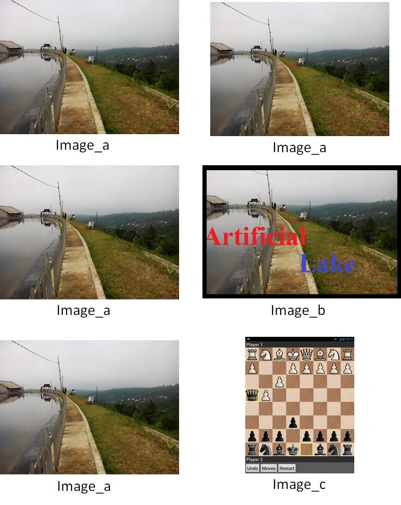
# First pair
hash1 = imagehash.average_hash(Image.open('D: /image_a.jpg'))
hash2 = imagehash.average_hash(Image.open('D:/ image_a.jpg'))
diff = hash1 - hash2
print(diff)
# 0

# Second pair
hash1 = imagehash.average_hash(Image.open('D: /image_a.jpg'))
hash2 = imagehash.average_hash(Image.open('D:/ image_b.jpg'))
diff = hash1 - hash2
print(diff)
# 6

# Third pair
hash1 = imagehash.average_hash(Image.open('D: /image_a.jpg'))
hash2 = imagehash.average_hash(Image.open('D:/ image_c.jpg'))
diff = hash1 - hash2
print(diff)
# 30

This is what the average image hash looks like

>imagehash.average_hash(Image.open('D:/image_a.jpg'))
array([[ True,  True,  True,  True,  True,  True,  True,  True],
       [ True,  True,  True,  True,  True,  True,  True,  True],
       [ True,  True,  True,  True,  True,  True,  True,  True],
       [False,  True, False, False, False, False, False, False],
       [ True,  True, False, False, False, False, False, False],
       [False, False, False,  True, False, False, False, False],
       [False, False, False,  True, False, False, False, False],
       [False, False, False, False, False, False, False, False]])

>imagehash.average_hash(Image.open('D:/image_b.jpg'))
array([[ True,  True,  True,  True,  True,  True,  True,  True],
       [ True,  True,  True,  True,  True,  True,  True,  True],
       [False,  True,  True,  True,  True, False, False, False],
       [ True,  True,  True, False, False, False, False, False],
       [ True,  True, False, False, False, False, False, False],
       [False, False, False,  True, False, False, False, False],
       [False, False, False,  True, False, False, False, False],
       [False, False, False, False, False, False, False, False]])

>imagehash.average_hash(Image.open('D:/image_c.png'))
array([[False, False, False, False, False, False, False, False],
       [ True,  True,  True,  True,  True,  True,  True,  True],
       [ True,  True,  True,  True,  True,  True,  True,  True],
       [ True,  True,  True,  True,  True,  True,  True,  True],
       [ True,  True,  True,  True,  True,  True,  True,  True],
       [ True,  True,  True,  True,  True,  True,  True,  True],
       [False, False, False, False,  True, False, False, False],
       [False, False, False, False, False, False, False, False]])

Text similarity

Text similarity can be assessed using natural language processing (PNL). There is 4 ways to compare the similarity of a pair of texts provided by the package “fuzzywuzzy”. The function in this package returns an integer value of 0 a 100. The highest value means the highest similarity.

1. fuzz.ratio – is the simplest comparison of texts. The fuzz.ratio value of “blue shirt” Y “blue shirt”. it is 95. It means that the two texts are similar or almost the same, but the point makes them a little different

from fuzzywuzzy import fuzz
fuzz.ratio('blue shirt','blue shirt.')
#95

Measurement is based on Levenshtein distance (named for Vladimir Levenshtein). Levenshtein distance measures how similar two texts are. Measure the minimum number of edits, how to insert, delete or replace a text in another text. The text “Blue shirt” requires only one edit to be “blue shirt”. It only takes a single point to be the same. Therefore, the Levenshtein distance is “1”. The fuzz relationship is calculated with this equation (len (a) + len (b) – lev) / ((len (a) + len (b), where len (a) y len (b) are the lengths of the first and second text, and lev is the Levenshtein distance The relation is (10 + 11 – 1) / (10 + 11) = 0,95 O 95%.

2. fuzz.partial_ratio: can detect if a text is part of another text. But it can't detect if the text is in a different order. The following example shows that “blue shirt” It is part of “clean blue shirt”, so fuzz.partial_ratio is 100. fuzz.ratio returns the value 74 because it only detects that there is a lot of difference between the two texts.

print(fuzz.ratio('blue shirt','clean blue shirt.'))
#74
print(fuzz.partial_ratio('blue shirt','clean blue shirt.'))
#100

3. Token_Sort_Ratio: can detect if a text is part of another text, even if they are in a different order. Fuzz.token_sort_ratio devuelve 100 for text “clean hat and blue shirt” Y “blue shirt and clean hat” because they actually mean the same thing, but they are in reverse order.

print(fuzz.ratio('clean hat and blue shirt','blue shirt and clean hat'))
#42
print(fuzz.partial_ratio('clean hat and blue shirt','blue shirt and clean hat'))
#42
print(fuzz.token_sort_ratio('clean hat and blue shirt','blue shirt and clean hat'))
#100

4. Token_Set_Ratio: can detect text similarity considering partial text, the order of the text and different lengths of text. You can detect that the text "clean hat" and "blue shirt" is part of the text "People want to wear blue shirt and clean hat" in a different order. In this studio, We only use "Token_Set_Ratio" since it is the most suitable.

print(fuzz.ratio('clean hat and blue shirt','People want to wear blue shirt and clean hat'))
#53
print(fuzz.partial_ratio('clean hat and blue shirt','People want to wear blue shirt and clean hat'))
#62
print(fuzz.token_sort_ratio('clean hat and blue shirt','People want to wear blue shirt and clean hat'))
#71
print(fuzz.token_set_ratio('clean hat and blue shirt','People want to wear blue shirt and clean hat'))
#100

The next cell will load the dataset from trainingTraining is a systematic process designed to improve skills, physical knowledge or abilities. It is applied in various areas, like sport, Education and professional development. An effective training program includes goal planning, regular practice and evaluation of progress. Adaptation to individual needs and motivation are key factors in achieving successful and sustainable results in any discipline.... and add hashing features, as well as the proportion of the token pool.

# load training set
trainingSet = pd.read_csv('D:/new_training_set.csv', index_col=0).reset_index()
# Compute imagehash difference
hashDiff = []
for i in trainingSet.index:
    hash1 = imagehash.average_hash(Image.open(path_img + trainingSet.iloc[i,2]))
    hash2 = imagehash.average_hash(Image.open(path_img + trainingSet.iloc[i,4]))
    diff = hash1 - hash2
    hashDiff.append(diff)
trainingSet = trainingSet.iloc[:-1,:]
trainingSet['hash'] = hashDiff
# Compute token_set_ratio
Token_test = []
for i in trainingSet.index:
    TokenSet = fuzz.token_set_ratio(trainingSet.iloc[i,1], trainingSet.iloc[i,3])
    TokenSet = (i, TokenSet)
    Token_tes.append(TokenSet)
dfToken = pd.DataFrame(token_test)
trainingSet['Token'] = dfToken

Below is the illustration of the training dataset. In reality, it is not the original dataset because the original dataset is not in english language. I create another data in English to understand it. Each row has two products. The columns “text_1” e “image 1” belong to the first product. The columns “text_2” e “image_2” belong to the second product. "Label" defines whether the matching products are the same (1) or not (0). Notice there are two other columns: “hash” Y “tokenSet”. These two columns are generated, not from the original data set, but from the previous code.

indexThe "Index" It is a fundamental tool in books and documents, which allows you to quickly locate the desired information. Generally, it is presented at the beginning of a work and organizes the contents in a hierarchical manner, including chapters and sections. Its correct preparation facilitates navigation and improves the understanding of the material, making it an essential resource for both students and professionals in various areas....	Text 1	image_1	text_2	image_2	Label	Hash	tokenSet
0	Blue shirt	Gdsfdfs.jpg	Blue shirt.	Safsfs.jpg	1	6	100
1	Clean hat	Fsdfsa.jpg	Clean pants	Yjdgfbs.jpg	0	25	71
2	mouse	Dfsdfasd.jpg	mouse	Fgasfdg.jpg	0	30	100
. . .	. . .	. . .	. . .	. . .	. . .	. . .	. . .

Apply machine learning

Now, we know that a lower Imagehash difference and a higher Token_Set_Ratio indicate that a pair of products is more likely to be the same. The lowest value of imagehash is 0 and the highest value of Token_Set_Ratio is 100. But, the question is how much are the thresholds. To set the thresholds, we can use the decision tree classifier.

A decision tree machine learning model is created using the training dataset. Machine learning algorithm will find image hash difference pattern and token set ratio of identical and different products. The decision tree is displayed for the cover image of this article. The following code creates a decision tree model with Python. (But, the display of the cover image is the decision tree generated with R because, in my opinion, R visualizes the decision tree in a more pleasant way). Later, will re-predict the training data set. Finally, we can get the precision.

# Create decision tree classifier: hash and token set
Dtc = DecisionTreeClassifier(max_depth=4) 
Dtc = Dtc.fit(trainingSet.loc[:,['hash', 'tokenSet']],
              trainingSet.loc[:,'Label'])
Prediction2 = Dtc.predict(trainingSet.loc[:,['hash', 'tokenSet']])
metrics.accuracy_score(trainingSet.loc[:,'Label'], Prediction2)

The decision tree is used to predict the classification of the training data set again. Precision is 0,728. In other words, the 72,8% of the training data set is predicted correctly.

From the decision tree, we can extract the information that if the Imagehash difference is less than 12, the product pair is classified as identical. If the Imagehash difference is greater than or equal to 12, we must check the Token_Set_Ratio value. El Token_Set_Ratio inferior a 97 confirm that the product pair is different. Otherwise, check again if the difference value of Imagehash. If the hash image difference is greater than or equal to 22, then the products are identical. On the contrary, the products are different.

Apply to test the dataset

Now, we will load the test data set, we will generate the difference Imagehash and Token_Set_Ratio, and finally we will predict if each pair of products matches.

# path to image
path_img = 'D:/test_img/'
# load test set
test = pd.read_csv('D:/new_test_set.csv', index_col=0).reset_index()
# hashDiff list
hashDiff = []
# Compute image difference
for i in test.index[:100]:
    hash1 = imagehash.average_hash(Image.open(path_img + test.iloc[i,2]))
    hash2 = imagehash.average_hash(Image.open(path_img + test.iloc[i,4]))
    diff = hash1 - hash2
    hashDiff.append(diff)
test['hash'] = hashDiff
# Token_set list
Token_set = []
# Compute text difference using token set
for i in test.index:
    TokenSet = fuzz.token_set_ratio(test.iloc[i,1], test.iloc[i,3])
    Token_set.append(TokenSet)
test['token'] = Token_set

After calculating the difference of Imagehash and Token_Set_ratio, the next thing you need to do is apply the decision tree for product match detection.

# Detecting product match
test['labelPredict'] = np.where(test['hash']<12, 1,
                               np.where(test['token']<97, 0,
                                        np.where(test['hash']>=22, 0, 1)))
# or
test['labelPredict'] = Dtc.predict(test[['hash','token']])

index	Text 1	image_1	text_2	image_2	Hash	tokenSet	labelPredict
0	pencil	Fdfgsdfhg.jpg	ballpoint	Adxsea.jpg	8	33	1
1	HDD	Sgytueyuyt.jpg	a good hard drive	Erewbva.jpg	20	100	1
2	draft	Sadssadad.jpg	stationary	Safdfgs.jpg	25	25	0
. . .	. . .	. . .	. . .	. . .	. . .	. . .	. . .

The table above is the illustration of the final result. The objective of this article is to demonstrate how to predict if two images and two texts are similar or the same. You may find that the machine learning model used is quite simple and there is no hyperparameter tuning or splitting of training and testing data. The other machine learning app, as tree-based set methods, can increase accuracy. But it is not our focus of discussion here. If you are interested in learning another tree-based machine learning more accurate than decision tree, look for an article here.

About the Author

Connect with me here https://www.linkedin.com/in/rendy-kurnia/

Related