
This article was published as part of the Data Science Blogathon.
Introduction
Table of Contents
-
What is linear regression?
-
Importance of linear regression in predictive analysis.
-
Practical application of linear regression using R.
-
Blood pressure and age dataset application.
What is a linear regression?
Simple linear regression analysis is a technique to find the association between two variables. Las dos variables involucradas son una variableIn statistics and mathematics, a "variable" is a symbol that represents a value that can change or vary. There are different types of variables, and qualitative, that describe non-numerical characteristics, and quantitative, representing numerical quantities. Variables are fundamental in experiments and studies, since they allow the analysis of relationships and patterns between different elements, facilitating the understanding of complex phenomena.... dependiente que responde al cambio y la variable independiente. Note that we are not calculating the dependence of the dependent variable on the independent variable, just the association.
For instance, a company is investing a certain amount of money in marketing a product and has also collected sales data over the years by analyzing the correlation in marketing budget and sales data, we can predict next year's sale if the company allocates a certain amount of money for the marketing department. The above prediction idea sounds magical, but it's pure statistics. Linear regression basically consists of fitting a straight line to our data set so that we can predict future events.
The line of best fit would be of the form:
Y = B0 + B1X
Where, Y – Dependent variable
X – Independent variable
B0 and B1 – Regression parameter
Prediction of blood pressure by age by regression in R
Regression line equation in our data set.
BP = 98,7147 + 0,9709 Age
Importing dataset
Import an Age vs Blood Pressure dataset that is a CSV file using the read.csv function () in R and store this dataset in a bp dataframe.
bp <- read.csv ("bp.csv")
Create data frame to predict values
Creation of a data frame that will store the age of 53 years. And this data frame will be used to predict blood pressure at 53 years after creating a linear regression model.
p <-  as.data.frame(53)
colnames(p) <- "Age"
Creando un Dispersion diagramThe scatter plot is a graphical tool used in statistics to visualize the relationship between two variables. It consists of a set of points in a Cartesian plane, where each point represents a pair of values corresponding to the variables analyzed. This type of chart allows you to identify patterns, Trends and possible correlations, facilitating data interpretation and decision-making based on the visual information presented.... usando la biblioteca ggplot2
Taking the help of the ggplot2 library in R, we can see that there is a correlation between blood pressure and age, as we can see that increasing age is followed by an increase in blood pressure.
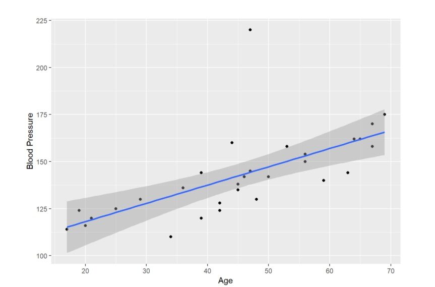
It is quite evident from the graph that the distribution on the graph is scattered in such a way that we can fit a straight line through the points.
Calculate the correlation between age and blood pressure
We can also verify our previous analysis that there is a correlation between blood pressure and age by taking the help of the function cor () in R which is used to calculate the correlation between two variables.
cor(bp$BP,bp$Age)
[1] 0,6575673
Create a linear regression model
Now, with the help of the lm function (), we are going to make a linear model. The lm function () has two attributes, first is a formula where we will use “BP ~ Age” because age is an independent variable and blood pressure is a dependent variable and the second is data, where we will give the name of the data frame that contains data which in this case is the bp data frame.
model <- lm(BP ~ Age, data = bp)
Summary of our linear regression model
summary(model)
Production:
##
## Call:
## lm(formula = BP ~ Age, data = bp)
##
## Residuals:
## Min 1Q Median 3Q Max
## -21.724 -6.994 -0.520 2.931 75.654
##
## Coefficients:
## Estimate Std. Error t value Pr(>|t|)
## (Intercept) 98.7147 10.0005 9.871 1.28e-10 ***
## Age 0.9709 0.2102 4.618 7.87e-05 ***
## ---
## Signif. codes: 0 '***' 0.001 '**' 0.01 * 0.05 '.' 0.1 ' ' 1
##
## Residual standard error: 17.31 on 28 degrees of freedom
## Multiple R-squared: 0.4324, Adjusted R-squared: 0.4121
## F-statistic: 21.33 on 1 and 28 DF, p-value: 7.867e-05
Interpretation of the model
## Coefficients:
## Estimate Std. Error t value Pr(>|t|)
## (Intercept) 98.7147 10.0005 9.871 1.28e-10 ***
## Age 0.9709 0.2102 4.618 7.87e-05 ***
## ---
## Signif. codes: 0 '***' 0.001 '**' 0.01 * 0.05 '.' 0.1 ' ' 1
B0 = 98.7147 (Y- intercept)
B1 = 0.9709 (Age coefficient)
BP = 98.7147 + 0.9709 Age
It means that a change in one unit in age will bring 0.9709 units to change in blood pressure.
Standard error It is the expected variability in the coefficient that captures the sampling variability, so the variation in the intersection can be up to 10.0005 and the variation in Age will be 0.2102 no more than that
Value T: the t-value is the coefficient divided by the standard error, it is basically how big is estimated in relation to the error, the greater the coefficient in relation to Std. error the higher the t-score and the t-score comes with a p-value because its distribution The p-value is how statistically significant the variable is for the model for a confidence level of the 95% we will compare this value with alpha which will be 0.05 , so in our case the p-value of the intersection and the Age is less than alpha (alfa = 0.05), this implies that both are statistically significant for our model.
## Residual standard error: 17.31 in 28 degrees of freedom
## Multiple R square: 0,4324, R squared fitted: 0,4121
## F statistic: 21,33 in 1 Y 28 DF, p value: 7,867e-05
Residual standard error or the standard error of the model is basically the average error for the model which is 17.31 in our case and means that our model can have an average error of 17.31 while predicting blood pressure. The smaller the error, the better the model will be when predicting.
Multiple R-square is the reason for (1- (sum of the squared error / sum of the total squared))
R squared fitted:
If we add variables, it does not matter if it is significant in the prediction or not, the value of R squared will increase, reason why adjusted R squared is used because if the aggregate variable is not significant for the model prediction, adjusted R value -squared will reduce, is one of the most useful tools to avoid overfitting the model.
F – statistics is the ratio between the mean square of the model and the mean square of the error, in other words, it is the reason how well the model is working and what is doing the error, and the higher the F value, the better the model is working compared to the error.
One is the degrees of freedom of the numerator of the F statistic and 28 is the degree of freedom of the errors.
Predict the value of blood pressure at 53 years
BP = 98,7147 + 0,9709 Age
The above formula will be used to calculate blood pressure at the age of 53 years and this will be achieved using the prediction function () first we will write the name of the linear regression model separating it by a comma giving the value of the new data set in p since Age 53 was previously saved in data frame p.
predict(model, newdata = p)
## 1
## 150.1708
Then, the predicted value of blood pressure is 150,17 to the 53 years.
How we have predicted blood pressure with the association of Age, now there may be more than one independent variable involved showing a correlation with a dependent variable called Multiple Regression.
Multiple linear regression model
Multilinear regression analysis is a statistical technique to find the association of multiple independent variables in the dependent variable.. For instance, the income generated by a company depends on several factors, including market size, the price, the promotion, the price of the competition, etc. Basically, the multiple linear regression model establishes a linear relationship between a dependent variable and multiple independent variables.
The multiple linear regression equation is as follows:
Y = B0 + B1X1 + B2X2 + .. + BnXk + E
Where
Y – Dependent variable
X – Independent variable
B0, B1, B3,. – Multiple linear regression coefficients
E- Error
Taking another example from the Wine dataset and with the help of AGST, HarvestRain let's predict the price of wine.
Importing the dataset
Using the read.csv function (), import dataset wine.csv and wine_test.csv into data frame wine and wine_test respectively.
wine <- read.csv("wine.csv")
wine_test <- read.csv("wine_test.csv")
Download the dataset from below
Find the correlation between different variables
Using the cor function () and the round function () we can round the correlation between all the variables in the wine dataset to two decimal places.
round(cor(wine),2)
Production:
Year Price WinterRain AGST HarvestRain Age FrancePop
## Year 1.00 -0.45 0.02 -0.25 0.03 -1.00 0.99
## Price -0.45 1.00 0.14 0.66 -0.56 0.45 -0.47
## WinterRain 0.02 0.14 1.00 -0.32 -0.28 -0.02 0.00
## AGST -0.25 0.66 -0.32 1.00 -0.06 0.25 -0.26
## HarvestRain 0.03 -0.56 -0.28 -0.06 1.00 -0.03 0.04
## Age -1.00 0.45 -0.02 0.25 -0.03 1.00 -0.99
## FrancePop 0.99 -0.47 0.00 -0.26 0.04 -0.99 1.00
Scattered plots
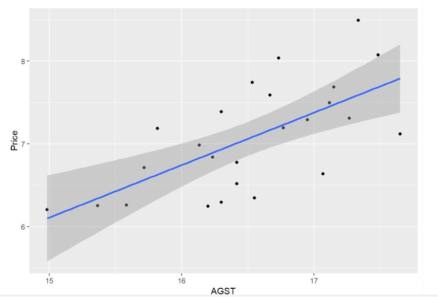
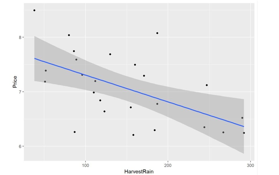
When using the ggplot2 library in R, create a scatterplot that can clearly show that AGST and wine price are highly correlated. In the same way, the scatter plotA scatter plot is a visual representation that shows the relationship between two numerical variables using points on a Cartesian plane. Each axis represents a variable, and the location of each point indicates its value in relation to both. This type of chart is useful for identifying patterns, Correlations and trends in the data, facilitating the analysis and interpretation of quantitative relationships.... entre HarvestRain y el precio del vino también muestra su correlación.
ggplot(wine,aes(x = AGST, y = Price)) + geom_point() +geom_smooth(method = "lm")
ggplot(wine,aes(x = HarvestRain, y = Price)) + geom_point() +geom_smooth(method = "lm")
Create a multilinear regression model
model1 <- lm(Price ~ AGST + HarvestRain,data = wine)
summary(model1)
Production:
##
## Call:
## lm(formula = Price ~ AGST + HarvestRain, data = wine)
##
## Residuals:
## Min 1Q Median 3Q Max
## -0.88321 -0.19600 0.06178 0.15379 0.59722
##
## Coefficients:
## Estimate Std. Error t value Pr(>|t|)
## (Intercept) -2.20265 1.85443 -1.188 0.247585
## AGST 0.60262 0.11128 5.415 1.94e-05 ***
## HarvestRain -0.00457 0.00101 -4.525 0.000167 ***
## ---
## Signif. codes: 0 '***' 0.001 '**' 0.01 * 0.05 '.' 0.1 ' ' 1
##
## Residual standard error: 0.3674 on 22 degrees of freedom
## Multiple R-squared: 0.7074, Adjusted R-squared: 0.6808
## F-statistic: 26.59 on 2 and 22 DF, p-value: 1.347e-06
Interpretation of the model
## Coefficients:
## Estimate Std. Error t value Pr(>|t|)
## (Intercept) -2.20265 1.85443 -1.188 0.247585
## AGST 0.60262 0.11128 5.415 1.94e-05 ***
## HarvestRain -0.00457 0.00101 -4.525 0.000167 ***
## Signif. codes: 0 '***' 0.001 '**' 0.01 * 0.05 '.' 0.1 ' ' 1
B0 = 98.7147 (Y- intercept)
B1 = 0.9709 (Age coefficient)
Price = -2.20265 + 0.60262 AGST - 0.00457 HarvestRain
It means that a change in a unit in AGST will bring 0,60262 units to change in price and a unit change in HarvestRain will bring 0,00457 units to change in price.
Standard error is the expected variability in the coefficient that captures the sampling variability, so the variation in the intersection can be up to 1.85443 and the variation in AGST will be 0.11128 and the variation in HarvestRain is 0.00101 no more than that
Value T: the t-value is the coefficient divided by the standard error, it is basically how big is estimated in relation to the error, the greater the coefficient in relation to Std. error the higher the t-score and the t-score comes with a p-value because it is a distribution.The p-value is how statistically significant the variable is for the model for a confidence level of the 95% we will compare this value with alpha to be 0.05, so in our case the p-value of the intersection, AGST and HarvestRain is less than alpha (alfa = 0.05), this implies that they are all statistically significant for our model.
## Residual standard error: 0.3674 in 22 degrees of freedom
## Multiple R square: 0,7074, R squared fitted: 0,6808
## F statistic: 26.59 in 2 Y 22 DF, p value: 1.347e-06
Residual standard error or the standard error of the model is basically the average error for the model which is 0.3674 in our case and means that our model can have an average difference of 0.3674 while predicting the price of wines. The smaller the error, the better the model will be when predicting.
Multiple R-square is the reason for (1- (sum of the squared error / sum of the total squared))
R squared fitted:
If we add variables, it does not matter if it is significant in the prediction or not, the value of R squared will increase, reason why adjusted R squared is used because if the aggregate variable is not significant for the model prediction, adjusted R value -squared will reduce, is one of the most useful tools to avoid overfitting the model.
F – statistics is the ratio between the mean square of the model and the mean square of the error, in other words, it is the reason how well the model is working and what is doing the error, and the higher the F value, the better the model is working compared to the error.
Two are the degrees of freedom of the numerator of the F statistic and 22 is the degree of freedom of the errors.
Prediction of values for our test suite
prediction <- predict(model1, newdata = wine_test)
Predicted values with the test data set
wine tasting
## Year Price WinterRain AGST HarvestRain Age FrancePop
## 1 1979 6.9541 717 16.1667 122 4 54835.83
## 2 1980 6.4979 578 16.0000 74 3 55110.24
prediction
## 1 2
## 6.982126 7.101033
Conclution
As we can see that from the available data set we can create a linear regression model and train that model, if enough data is available, we can accurately predict new events or, in other words, future results.





