
This article was published as part of the Data Science Blogathon
Introduction
If you are reading this article, I guess you are already in the world of data science and have an idea about machine learning. If that is not the case, No problem. I will start with the basic terminologies that you need to know before understanding the main topic of discussion, namely, linear regression.
This article will cover everything you need to know about linear regression., the first data science machine learning algorithm.
Table of Contents
- Brief introduction to machine learning and its types
- Understanding linear regression
- Linear regression assumptions.
- How to deal with the violation of the assumptions
- Evaluation metrics for regression problems
Introduction to machine learning
Machine learning is a branch of artificial intelligence (HE) focused on building applications that learn from data and improve accuracy over time without being programmed to do so.
Types of machine learning:
Supervised machine learning: It is an ML technique in which models are trained with labeled data, namely, is provided a variableIn statistics and mathematics, a "variable" is a symbol that represents a value that can change or vary. There are different types of variables, and qualitative, that describe non-numerical characteristics, and quantitative, representing numerical quantities. Variables are fundamental in experiments and studies, since they allow the analysis of relationships and patterns between different elements, facilitating the understanding of complex phenomena.... output in this type of problems. Here, models find mapping function to map input variables to output variable or labels.
Regression and classification Problems are part of supervised machine learning.
Unsupervised machine learning: It is the technique in which the models do not receive the labeled data and have to find the patterns and the structure in the data to know the data.
Grouping and association Algorithms are part of unsupervised ML.
Understanding linear regression
In the simplest words Linear regression is the supervised machine learning model in which the model finds the linear line of best fit between the independent and dependent variable namely, find the linear relationship between the dependent and independent variables.
Linear regression is of two types: Simple and multiple. Simple linear regression is where only one independent variable is present and the model has to find its linear relationship with the dependent variable
While in Multiple linear regression there is more than one independent variable for the model to find the relationship.
Simple linear regression equation, where bO is the intersection, b1 is coefficient or slope, x is the independent variable and y is the dependent variable.
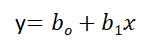

Multiple linear regression equation, where bO is the intersection, b1,B2,B3,B4…,BNorth are coefficients or slopes of the independent variables x1,X2,X3,X4…,XNorth and y is the dependent variable.


The main objective of a linear regression model is to find the linear line that best fits and the optimal values of intersection and coefficients in a way that minimizes the error.
The error is the difference between the actual value and the predicted value and the goal is to reduce this difference.
Let's understand this with the help of a diagram.
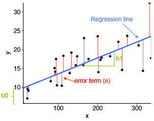
Image source: statistical tools for high-performance data analysis
In the diagram above,
- x is our dependent variable that is plotted on the x-axis and y is the dependent variable that is plotted on the y-axis.
- The black points are the data points, namely, the actual values.
- BO is the intersection that is 10 and b1 is the slope of the variable x.
- The blue line is the line of best fit predicted by the model, namely, predicted values are on the blue line.
The vertical distance between the data point and the regression line is known as the error or residual. Each data point has a remainder and the sum of all the differences is known as the sum of the residuals / mistakes.
Mathematical approach:
Residual / Error = Actual values – Predicted values
Sum of residuals / errors = Sum (expected actual values)
Square of the sum of the residuals / errors = (Sum (expected actual values))2
namely
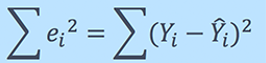
For a deep understanding of the mathematics behind linear regression, see attachment video explanation.
Linear regression assumptions
The basic assumptions of linear regression are as follows:
1. Linearity: Establishes that the dependent variable Y must be linearly related to the independent variables. This assumption can be verified by drawing a scatter diagram between both variables.
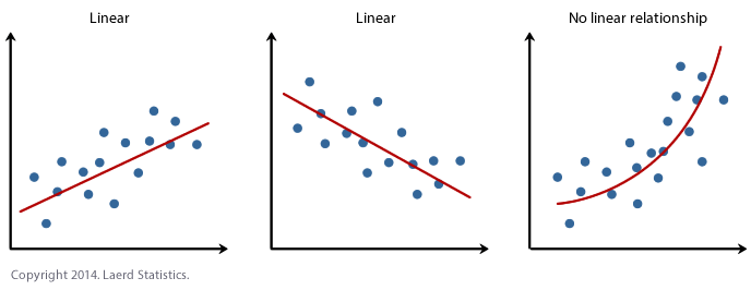
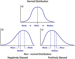
2. Normal: Variables X and Y must have a normal distribution. Histograms can be used, KDE graphs and QQ graphs to check the normality assumption.
See my attached blog for a detailed explanation on how to check for normality and transform variables that violate the assumption.
Source: https://heljves.com/gallery/vol_1_issue_1_2019_8.pdf
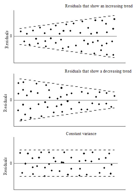
3. Homoscedasticity: The variance of the error terms must be constant, namely, the dispersion of the residuals must be constant for all values of X. This assumption can be verified by drawing a residual graph. If the assumption is violated, the dots will form a funnel shape, otherwise they will be constant.
Source: OriginLab
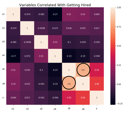
4. Independence / No multicollinearity: The variables must be independent of each other, namely, there should be no correlation between the independent variables. To verify the assumption, we can use a correlation matrix or a VIF score. If the VIF score is greater than 5, the variables are highly correlated.
In the image below, there is a high correlation between the variables x5 and x6.
Source: towards data science
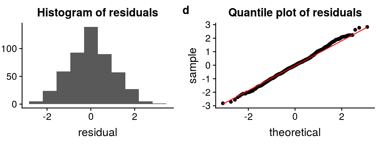
5. the error terms should be distributed normally. QQ charts and histograms can be used to check the distribution of error terms.
Source: http://rstudio-pubs-static.s3.amazonaws.com
6. No autocorrelation: The error terms must be independent of each other. Autocorrelation can be tested using the Durbin Watson test. The null hypothesis assumes that there is no autocorrelation. The value of the test is between 0 Y 4. If the test value is 2, no autocorrelation.
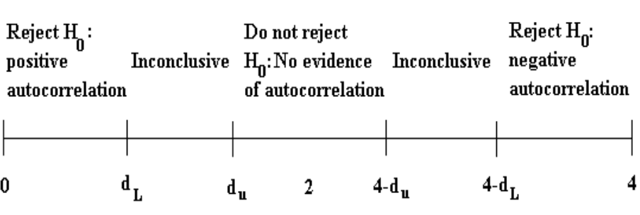
Source: itfeature.com
How to deal with the violation of any of the assumptions
Violation of the assumptions leads to a decrease in the precision of the model, so the predictions are not accurate and the error is also high.
For instance, if the independence assumption is violated, the relationship between the independent and dependent variable cannot be determined precisely.
There are various methods and techniques available to deal with the violation of the assumptions. Let's analyze some of them below.
Violation of the assumption of normality of variables or error terms
To treat this problem, we can transform the variables to the normal distribution using various transformation functions like logarithmic transformation, Reciprocal Box-Cox Transformation.
All functions are discussed in this article of mine: How to transform to normal distribution
Violation of the multicollinearity assumption
It can be treated by:
- Do nothing (if there is no major difference in precision)
- Eliminating some of the highly correlated independent variables.
- Derive a new characteristic by linearly combining the independent variables, how to add them or perform some mathematical operation.
- Carrying out an analysis designed for highly correlated variables, such as principal component analysis.
Evaluation metrics for regression analysis
To understand the performance of the regression model, an evaluation of the model is necessary. Some of the evaluation metrics used for regression analysis are:
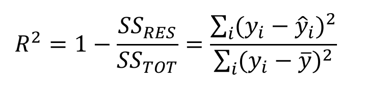
1. R squared or coefficient of determination: The most used metric for model evaluation in regression analysis is R squared. It can be defined as a ratio of variation to total variation. The value of R squared is between 0 Y 1, the closer to 1, the better the model.
Source: medium.datadriveninvestor.com
where SSRES is the residual sum of squares and SSTOT is the total sum of squares
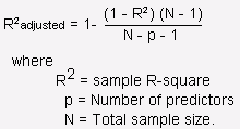
2. R squared fitted: It is the improvement of R squared. The problem / drawback of R2 is that as features increase, the value of R2 also increases, which gives the illusion of a good model. Then, Adjusted R2 solves the R2 issue. It only considers the features that are important to the model and shows the actual improvement of the model.
Adjusted R2 is always less than R2.
Source: stats.stackexchange.com
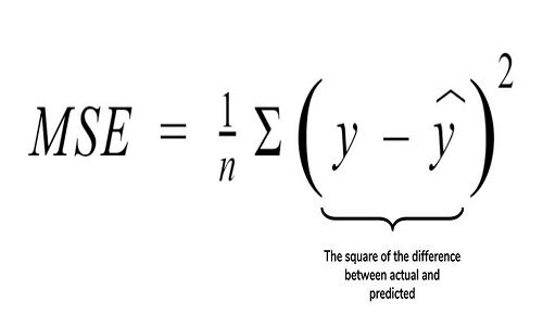
3. Root mean square error (MSE): Another common metric for evaluation is the root mean square error., which is the mean of the squared difference of the real values versus the predicted ones.
Source: cppsecrets.com
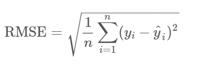
4. Root mean square error (RMSE): It is the root of MSE, namely, the root of the mean difference of the actual and predicted values. RMSE penalizes big mistakes, while MSE does not.
Source: community.qlik.com
Final notes
We have covered most of the regression model concepts on this blog. If you want to explore more about the math behind the model, see the links attached to the blog.
Please, feel free to connect with me on LinkedIn and share your valuable input. Please, check out my other articles here.
About the Author :
Soy Deepanshi Dhingra, I currently work as a data science researcher and have a background in analytics, exploratory data analysis, machine learning and deep learningDeep learning, A subdiscipline of artificial intelligence, relies on artificial neural networks to analyze and process large volumes of data. This technique allows machines to learn patterns and perform complex tasks, such as speech recognition and computer vision. Its ability to continuously improve as more data is provided to it makes it a key tool in various industries, from health....
This article was published as part of the Data Science Blogathon





