
Overview
- Get an introduction to logistic regression using R and Python
- Logistic regression is a popular classification algorithm used to predict a binary outcome.
- There are several metrics to evaluate a logistic regression model, as matrix of confusion, curva AUC-ROC, etc.
Introduction
Every machine learning algorithm works best under a given set of conditions. Make sure your algorithm fits the assumptions / requirements ensures superior performance. No algorithm can be used in any condition. For instance: Have you ever tried to use linear regression in a variableIn statistics and mathematics, a "variable" is a symbol that represents a value that can change or vary. There are different types of variables, and qualitative, that describe non-numerical characteristics, and quantitative, representing numerical quantities. Variables are fundamental in experiments and studies, since they allow the analysis of relationships and patterns between different elements, facilitating the understanding of complex phenomena.... categorical dependent? Do not even try! Because you will not be appreciated for getting extremely low values of the adjusted R² and F statistic.
However, in such situations, you should try using algorithms like Logistic Regression, Decision trees, SVM, Random forest, etc. For a quick overview of these algorithms, I will recommend reading: Machine learning algorithm basics.
With this post, I provide you with useful knowledge about logistic regression in R. Once you have mastered linear regression, this is the natural next step on your journey. It is also easy to learn and implement, but you must know the science behind this algorithm.
I tried to explain these concepts in the simplest way possible. Let us begin.
Project to apply Logistic RegressionProblem StatementHR analytics is revolutionizing the way HR departments operate, leading to higher efficiency and better results overall. Human resources have been using the analyticsAnalytics refers to the process of collecting, Measure and analyze data to gain valuable insights that facilitate decision-making. In various fields, like business, Health and sport, Analytics Can Identify Patterns and Trends, Optimize processes and improve results. The use of advanced tools and statistical techniques is essential to transform data into applicable and strategic knowledge.... during years. But nevertheless, the compilation, data processing and analysis has been largely manual and, dada la naturaleza de la dinámica de los recursos humanos y los KPIKPIs, o Key performance indicators, These are metrics used by organizations to evaluate their success in achieving specific goals. These indicators allow you to monitor progress and make informed decisions. There are different types of KPIs, which may vary depending on the sector and the strategic objectives of the company. Its correct implementation is essential to improve the efficiency and effectiveness of operations.... de recursos humanos, the focus has been restricting to human resources. Therefore, it's surprising hr departments have come to realize the usefulness of machine learning so late in the game. This is an opportunity to test predictive analytics to identify employees most likely to be promoted. |
What is logistic regression?
Logistic regression is a classification algorithm. Used to predict a binary outcome (1/0, Yes / No, True / Fake) given a set of independent variables. To represent a binary result / categorical, we use dummy variables. You can also think of logistic regression as a special case of linear regression when the outcome variable is categorical., where we use the logarithm of probabilities as the dependent variable. In simple words, predicts the probability of occurrence of an event by fitting the data to a logit function.
Derivation of the logistic regression equation
Logistic regression is part of a larger class of algorithms known as the generalized linear model. (glm). In 1972, Nelder and Wedderburn proposed this model in an effort to provide a means of using linear regression for problems that were not directly suitable for applying linear regression.. In fact, proposed a class of different models (linear regression, ANOVA, Poisson regression, etc.) that included logistic regression as a special case.
The fundamental equation of the generalized linear model is:
g(E(Y)) = α + βx1 + γx2
Here, g () is the link function, E (Y) is the expectation of the target variable and α + βx1 + γx2 is the linear predictor (a, b, γ to be predicted). The role of the link function is “link” the expectation of y to the linear predictor.
Important points
- GLM does not assume a linear relationship between dependent and independent variables. But nevertheless, assumes a linear relationship between the link function and the independent variables in the logit model.
- The dependent variable does not need to be normally distributed.
- Does not use OLS (Ordinary least square) for the estimation of parametersThe "parameters" are variables or criteria that are used to define, measure or evaluate a phenomenon or system. In various fields such as statistics, Computer Science and Scientific Research, Parameters are critical to establishing norms and standards that guide data analysis and interpretation. Their proper selection and handling are crucial to obtain accurate and relevant results in any study or project..... However, uses maximum likelihood estimation (MLE).
- Errors must be independent but not normally distributed.
Let's understand more with an example:
We are provided with a sample of 1000 customers. We need to predict the probability that a customer will buy (Y) a particular magazine or not. As you can see, we have a categorical result variable, we will use logistic regression.
To get started with logistic regression, I will first write the simple linear regression equation with the dependent variable enclosed in a link function:
g(Y) = βo + b(Age) ---- (a)
Note: To facilitate understanding, I have considered ‘Age’ as independent variable.
In the logistic regression, we are only concerned with the probability of the dependent variable of the result (success or failure). As described above, g () is the link function. This function is established by two things: probability of success (p) and probability of failure (1-p). p must meet the following criteria:
- It should always be positive (since p> = 0)
- It must always be less than equal to 1 (since p <= 1)
Now, we will simply satisfy these 2 conditions and get to the core of the logistic regression. To set the link function, we will denote g () with 'p’ initially and eventually we will end up deriving this function.
Since the probability must always be positive, we will put the linear equation in exponential form. For any value of slope and dependent variable, the exponent of this equation will never be negative.
p = exp(βo + b(Age)) = e^(βo + b(Age)) ------- (b)
For the probability to be less than 1, we must divide p by a number greater than p. This can be done simply by:
p = exp(βo + b(Age)) / exp(βo + b(Age)) + 1 = e^(βo + b(Age)) / e^(βo + b(Age)) + 1 ----- (c)
Using (a), (b) Y (c), we can redefine probability as:
p = e^y/ 1 + e ^ y --- (d)
where p is the probability of success. This (d) is the Logit function
If p is the probability of success, 1-p will be the probability of failure which can be written as:
q = 1 - p = 1 - (e ^ y / 1 + e ^ y) --- (e)
where q is the probability of failure
By dividing, (d) / (e), we obtain,
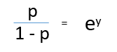
After taking the record on both sides, we obtain,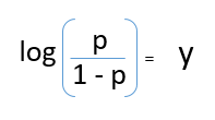
log (p / 1-p) is the link function. The logarithmic transformation of the result variable allows us to model a non-linear association in a linear way.
After substituting the value of y, we will get:
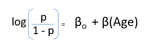
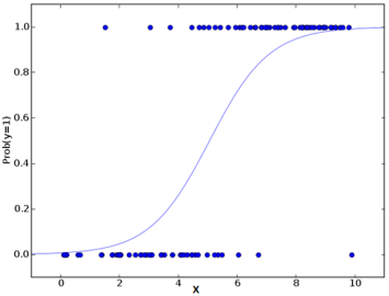
This is the equation used in Logistic Regression. Here (p / 1-p) is the odd reason. When the logarithm of the odd ratio is determined to be positive, the probability of success is always higher than 50%. Below is a typical logistic model graph. You can see that the probability never drops below 0 and above 1.
Performance of the logistic regression model
To evaluate the performance of a logistic regression model, we must consider some metrics. Regardless of the tool (SAS, R, Python) in which I would work, always look:
1. AIC (Akaike information criteria) – The analogous metric of adjusted R2 in logistic regression is AIC. AIC is the adjustment measure that penalizes the model for the number of coefficients of the model. Therefore, we always prefer the model with a minimum value of AIC.
2. Null deviation and residual deviation – The null deviation indicates the response predicted by a model with nothing more than an intersection. Lower the value, better model. The residual deviation indicates the response predicted by a model when adding independent variables. Lower the value, better model.
3. Confusion matrix: It is nothing more than a tabular representation of the actual values versus the predicted ones.. This helps us find the accuracy of the model and avoid overfitting.. This is what this looks like:
 Source: (plug – n – score)
You can calculate the precision of your model with:

From the confusion matrix, specificity and sensitivity can be derived as illustrated below:
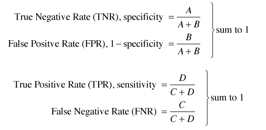
Specificity and sensitivity play a crucial role in the derivation of the ROC curve..
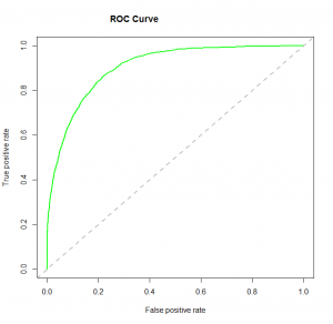
4. ROC curve: The operating characteristic of the receiver (ROC) summarizes the performance of the model by evaluating the tradeoffs between the rate of true positives (sensitivity) and the false positive rate (1 specificity). To graph ROC, it is advisable to assume p> 0.5 since we are more concerned with the success rate. ROC summarizes the predictive power for all possible values of p> 0.5. The area under the curve (AUC), called indexThe "Index" It is a fundamental tool in books and documents, which allows you to quickly locate the desired information. Generally, it is presented at the beginning of a work and organizes the contents in a hierarchical manner, including chapters and sections. Its correct preparation facilitates navigation and improves the understanding of the material, making it an essential resource for both students and professionals in various areas.... precision (A) or concordance index, is a perfect performance metric for the ROC curve. The larger the area under the curve, the better the predictive power of the model. Below is a sample ROC curve. The ROC of a perfect predictive model has TP equal to 1 and FP equal to 0. This curve will touch the upper left corner of the graph..
Note: For model performance, you can also consider the probability function. It is so named because it selects the values of the coefficients that maximize the probability of explaining the observed data. Indicates goodness of fit when its value approaches one and a poor fit of the data when its value approaches zero.
Logistic regression model in R and Python
R code is provided below, but if you are a python user, here is an amazing code window to build your logistic regression model. No need to open Jupyter, puede hacerlo todo aquí:
Teniendo en cuenta la disponibilidad, construí este modelo en nuestro problema de práctica: el conjunto de datos de Dressify. Puedes descargarlo here.
Sin profundizar en la ingeniería de características, aquí está el script del modelo de regresión logística simple:
set('C:/Users/manish/Desktop/dressdata')
#load data
train <- read.csv('Train_Old.csv')
#create training and validation data from given data
install.packages('caTools')
library(caTools)
set.seed(88)
split <- sample.split(train$Recommended, SplitRatio = 0.75)
#get training and test data
dresstrain <- subset(train, split == TRUE)
dresstest <- subset(train, split == FALSE)
#logistic regression model
model <- glm (Recommended ~ .-ID, data = dresstrain, family = binomial)
summary(model)
predict <- predict(model, type="response")
#confusion matrix
table(dresstrain$Recommended, predict > 0.5)
#ROCR Curve
library(ROCR)
ROCRpred <- prediction(predict, dresstrain$Recommended)
ROCRperf <- performance(ROCRpred, 'tpr','fpr')
plot(ROCRperf, colorize = TRUE, text.adj = c(-0.2,1.7))
#plot glm
library(ggplot2)
ggplot(dresstrain, aes(x=Rating, y=Recommended)) + geom_point() +
stat_smooth(method="glm", family="binomial", se=FALSE)
This data requires a lot of cleaning and feature engineering. The scope of this article restricted me to keep the example focused on the construction of the logistic regression model.. These data are available to practice. I recommend that you work on this problem. There is much to learn.
Final notes
At this stage, you will already know the science behind logistic regression. I have seen many times that people know the use of this algorithm without having knowledge about its core concepts. I have tried my best to explain this part in the simplest way possible. The previous example only shows the skeleton of using logistic regression in R. Before really approaching this stage, you must invest your crucial time in feature engineering.
What's more, I recommend that you work on this set of problems. You would explore things that you may not have faced before.
Did I miss something important? Do you find helpful this article? Share your opinions / thoughts in the comment section below.





