Markov chain | Characteristics and applications of the Markov chain

This article was published as an entry for the Data Science Blogathon.

Introduction

Markov chains are exceptionally useful for modeling a discrete-time discrete-space stochastic process of various domains such as finance. (stock price movement), NLP algorithms (finite state transducers, Hidden Markov model for POS labeling), or even in physical engineering ( Brownian movement).

Taking into account the immense usefulness of this concept in various domains and its fundamental importance for a significant number of algorithms in data science, we will cover in this article the following aspects of the Markov Chain:

1. Markov chain formulation and intuitive explanation
2. Aspects and characteristics of a Markov chain
3. Applications and use cases

Markov chain formulation and intuitive explanation

To understand what a Markov chain is, first let's see what a stochastic process is, since the Markov chain is a special type of stochastic process.

A stochastic process is defined as a collection of random variables X = {X_t: t∈T} defined in a common probability space, taking values ​​in a common set S (state space), and indexed by a set T, Not often [0, ∞) and thought of as time (discrete or continuous respectively) (Oliver, 2009). It means that we have observations at a certain time and the outcome is a random variableIn statistics and mathematics, a "variable" is a symbol that represents a value that can change or vary. There are different types of variables, and qualitative, that describe non-numerical characteristics, and quantitative, representing numerical quantities. Variables are fundamental in experiments and studies, since they allow the analysis of relationships and patterns between different elements, facilitating the understanding of complex phenomena..... Simply put, a stochastic process is any process that describes the evolution in time of a random phenomenon.

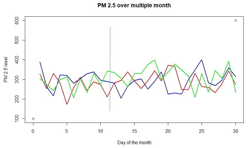
Consider the graph above of concentration of PM (particulate matter) 2.5 in the air over a city for different months. Each of the colored lines -red, blue, and green – (called sample-path) represents a random function of time. Also, consider any day (say 15th of every month), it represents a random variable. Thus it can be considered as a Stochastic process, i.e a process that takes different functional inputs at different times. This particular example is a case for discrete-time (as time is not continuous, observed once a day) with a continuous state (it can take any positive value, not necessarily an integer).

Now that we have a basic intuition of a stochastic process, let’s get down to understand one of the most useful mathematical concepts for Data Science: Markov Chains!

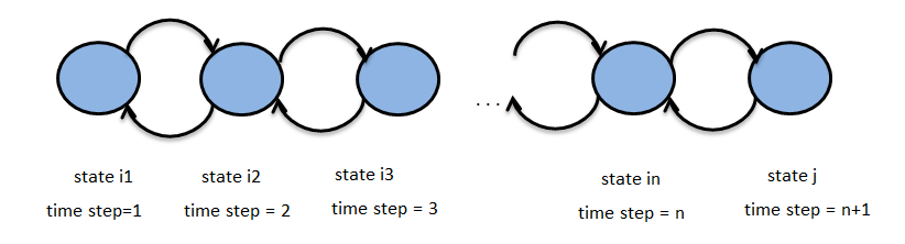
The above figure represents a Markov chain, with states i₁, i₂ ,… , i_n , j for time steps 1, 2, .., n+1. Let {WITH_n}_n∈N be the above stochastic process with state space S. N here is the set of integers and represents the time set and Z_n represents the state of the Markov chain at time n. Suppose we have the property :

P(WITH_n+1 = j | WITH_n = i_n , WITH_n-1 = i_n-1 , … , WITH₁ = i₁) = P(WITH_n+1 = j | WITH_n = i_n)

then {WITH_n}_n∈N is called a Markov Chain.

This term P(WITH_n+1 = j | WITH_n= i_n) is called transition probability. Thus we can intuitively see that in order to describe Markov Chain probabilistically, we need (a) the initial state distribution and (b) transition probabilities.

Let’s take the Markov Chain shown below to understand these two terms more formally,

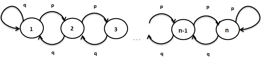
In the Markov chain above, states are 1, 2, …, n and the probability of going from any state k to k+1 (for k =1, 2, …, n-1) is p and going from state k to k-1 is q, where"WHERE" is a term in English that translates as "where" in Spanish. Used to ask questions about the location of people, Objects or events. In grammatical contexts, it can function as an adverb of place and is fundamental in the formation of questions. Its correct application is essential in everyday communication and in language teaching, facilitating the understanding and exchange of information on positions and directions.... q = 1-p.

• The initial state distribution is defined as

Pi₍₀₎ = [P(X₀=1), P(X₀=2), … , P(X₀ = n)]

The previous expression is a row vector with element that denotes the probability that the Markov chain has the state i, where i = 1, 2,…, n. All the elements of this vector add up to 1.

• the transition probability matrix it is as shown below :

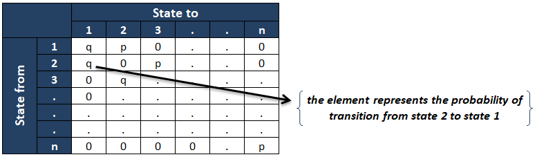
El ij^th element of the transition probability matrix represents the the conditional probability the string is in state j since it was in state i at the previous time. If the transition probability matrix does not depend on “n” (weather), then the string is called the Homogeneous Markov chain.

Aspects and characteristics of a Markov chain

In this section, we will see the following main aspects of a Markov chain:

• Time of first hit: g_l(k)
• Average impact time (absorption time): h_A(k)

The purpose of the previous two analyzes is that if we have a set of desired states (let's say A), and we want to calculate how long it will take to reach the desired state.

First hour of blow

Imagine, if we want to know the probability (conditional) that our Markov chain, which begins in some initial state k, reach state l (one of many desired states in A) as long as it reaches any state in A. How we do it? that?

Let's understand by defining some basic terms. Let T_A be the earliest time it takes to reach any of the states in set A and k be some state in state space but not in A.

Let g_l(k) be defined as the conditional probability of reaching state l at time T_A from state k.

Now, using the Markov property, Let's consider passing the state in time = 0 to the state in time = T_A how to pass the state in time = 0 to the state in time = 1 and then go from state to time = 1 to the state in time = TA. The same is represented below:

The above equation can be interpreted graphically as shown below, namely, in the first step you can go from state k to any of the states m in one step and then go in T_A-1 passage from state m to desired state l.

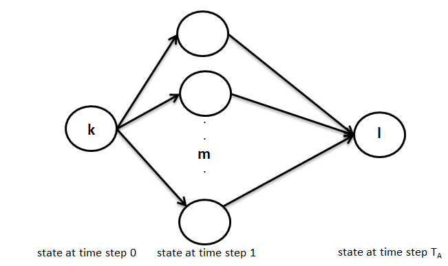
Now, the first term can be represented as g_l(m) and the second term represents the transition probability from state k to state m

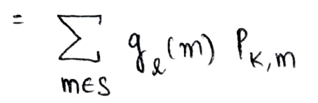
This is the recursive way we calculate the desired probability and the approach used above is called First step analysis (as we analyze it in terms of the first step the state takes in time = 0 to the state in time = 1)

Average hit time

Using a similar approach as above, we can also calculate the average time (expected) to achieve a desired set of states (let's say A) from a state k out of A.

Definamos h_A(k) as the expected time required to reach a set A from state k. This is defined as shown below:

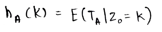
Now that we know what the first step analysis is, Why not use it again?

Then, now we write the expectation term in terms of the first step (namely, reach state Z₁) As shown below:

Now, using the Markov property, we can eliminate the Z₀ term as we know the state in Z₁. The second term in the above product is the transition probability from state k to state l (we've seen this concept so much that now it feels like a calculation 2 + 2 = 4 🙂)

Note that the expectation term below is in terms of Z₁ (and not Z₀) and therefore we cannot write it directly as h_A(k). Therefore, we use a math trick, we add 1 in expectation and we subtract 1 also so that we can mathematically write the state as Z₀ = l

And now we can write it as h_A(k).

This is the recursive way we calculate the desired Expectation!!

Now we know the fundamental approach to derive any Markov property with the two new tools that we have: Understanding of transition probability matrix Y First-step analysis approach.

Applications and use cases

Since we are now comfortable with the concept and aspects of a Markov chain, Let's explore and intuitively understand the following application and use cases of Markov chains.

• PNL: hidden Markov model for point of sale labeling
• Random walk like a Markov chain

PNL: hidden Markov model for point of sale labeling

Labeling of part of speech (POS) is an important application of NLP. The goal in these problems is to tag each word in a given sentence with an appropriate POS (noun, verb, adverb, etc.). In the model, we have label transition probabilities, namely, since the label of the previous word is said t_i-1, The t_I will be the label of the current word. And the second concept of the model is the probability that given the label of the current word is t_I, the word will be w_I. To put it more clearly: the hidden Markov model is a type of Generative models (sets) in which the hidden states (here POS labels) are considered given and the observed data are considered generated.

The t_I on the figure"Figure" is a term that is used in various contexts, From art to anatomy. In the artistic field, refers to the representation of human or animal forms in sculptures and paintings. In anatomy, designates the shape and structure of the body. What's more, in mathematics, "figure" it is related to geometric shapes. Its versatility makes it a fundamental concept in multiple disciplines.... siguiente se refiere a las etiquetas POS del estado yw_I refers to the words issued by the states.

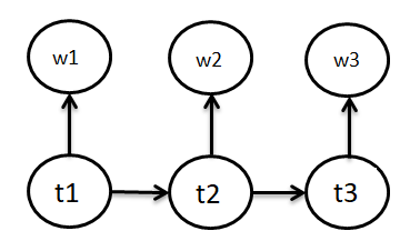
Now, let's take a closer look at the element of the model to see the Markov process in it even more clearly. The elements of the hidden Markov model are:

• A set of states: here POS Labels
• The output of each state: here ‘word’
• initial state: here I start the sentence
• State transition probability: here P (t_North | t_n-1)

Besides being very useful in this aspect of NLP, finite state transducers and many other algorithms are based on Markov chains.

Random walk

Another interesting phenomenon is that of Random walk, which again is a Markov Chain.

Let's consider the random walk, as shown above, namely, movement one step forward from any state can occur with probability p and movement back one step can occur with probability q. Here the forward movement from state k to k + 1 depends only on state k and, Thus, Random Walk is a Markov chain.

Now, let's step forward and understand the random walk as a Markov chain using simulation. Here we consider the case of the one-dimensional walk, where the person can step forward or backward of any size (size> = 1) with equal probability.

Here, I have traced 30 random walks to develop intuition around the phenomenon. Here, the initial state of the Markov chain is 0 (zero cumulative steps initially). Things to keep in mind are:

• State space and set time are both discrete (integers)
• It is visually clear that at any given time step, the next state is determined only by the current state and the time steps behind the current time step do not help to predict where the chain state will be in the next time step.
• Since the probability of forward movement is the same as that of backward movement, the expected value of the cumulative number of steps is 0.

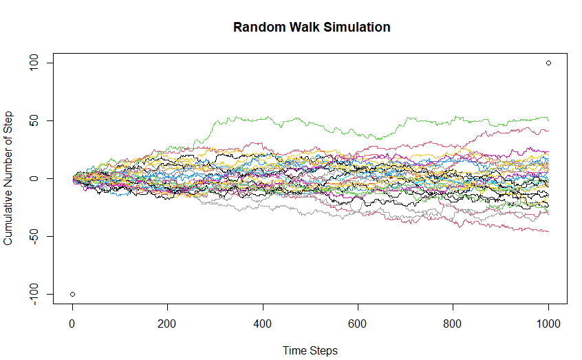
The code to simulate a basic random walk in R is given below:

plot(c(0,1000),c(-100,100), xlab = "Time Steps", ylab = "Cumulative Number of Step" , main = " Random Walk Simulation")
for (i in 1:30) {
  x <- as.integer(rnorm(1000))
  lines(cumsum(x), type = "l", col=sample(1:10,1)) 
}

The Markov chain is a very powerful and effective technique for modeling a stochastic process of discrete time and space.. The understanding of the two previous applications together with the explained mathematical concept can be used to understand any type of Markov process.

Note about the author: I am a PGDBA student (Graduate Diploma in Business Analysis) and IIM Calcutta, IIT Kharagpur and ISI Kolkata, and I have completed my B.TECH from IIT DELHI and have a work experience of ~ 3,5 years in advanced analytics.

Feel free to reach out for any discussion on the subject at Parth Tyagi | LinkedIn or write me an email to [email protected]

The media shown in this article is not the property of DataPeaker and is used at the author's discretion.

Related