Point estimators | Guide to point estimators in statistics

Introduction

Estimation theory Y Hypothesis testing are the very important concepts of Statistics that are widely used by Statistics, Machine learning engineers, Y Data scientists.

Then, in this post, we will discuss point estimators in estimation theory of statistics.

Table of Contents

1. Estimators and estimators

2. What are point estimators?

3. What is the random sample and statistic?

4. Two common statistics used:

• Average sample
• Sample variance

5. Properties of point estimators

• Impartiality
• Efficient
• Consistent
• Enough

6. Common Methods for Finding Point Estimates

7. Point estimate vs. interval estimate

Estimation and estimators

Let X be a random variable with distribution F_X(x; θ), where θ is an unknown parameter. A random sample, X₁, X₂, –, X_North, of size n taken at X.

The point estimation problem is selecting a statistic, g (X₁, X₂, —, X_North), that best estimates the parameter θ.

Once observed, the numerical value of g (x₁, X₂, —, X_North) it's called estimation and statistics g (X₁, X₂, —, X_North) it's called estimator.

What are point estimators?

Point estimators are defined as the functions that are used to find an approximate value of a population parameter from random samples of the population.. They take the help of sample data from a population to establish a point estimate or statistic that serves as the best estimate of an unknown parameter of a population.

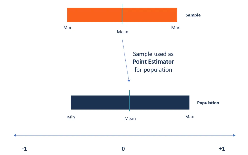
Image source: Google images

Very often, existing methods for finding the parameters of large populations are unrealistic.

As an example, when we want to find the average height of people attending a conference, it will be impossible to collect the exact height of all the conference towns in the world. However, a statistician can use the point estimator to estimate the population parameter.

Random sample and statistics

Aleatory sample: A set of IID (independently and identically distributed) random variables, X₁, X₂, X₃, —, X_North established in the same sample space is called a random sample of size n.

Statistics: A function from a random sample is called a statistic (if not dependent on any unknown entity)

As an example, X₁+ X₂+ —— + X_North, X₁²X₂+ e^X3, X₁– X_North

Sample mean and sample variance

Two important statistics:

Let x₁, X₂, X₃, —, X_North be a random sample, then:

The sample mean is denoted by X, and the sample variance is denoted by s²

Here x̄ ys² they are called the sample parameters.

Population parameters are indicated through:

σ² = population variance and µ = population mean

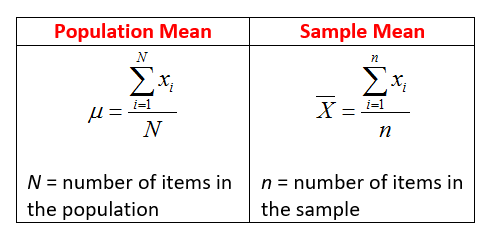
Fig. Population and sample mean

Image source: Google images

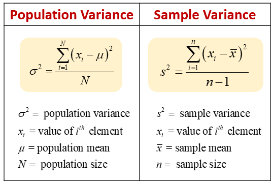
Fig. Sample population and variance

Image source: Google images

Characteristics of the sample mean:

E (x̄) = 1 / n (Σ E (X_I)) = 1 / n (nµ) = µ

Where (x̄) = 1 / n²(Σ Var (X_I)) = 1 / n² (nσ²) = σ²/North

Characteristics of the sample variance:

s² = 1 / (n-1) (Σ (x_I– X )² ) = 1 / (n-1) (Σ x_I² – 2x̄ Σ x_I + nx̄² ) = 1 / (n-1) (Σ x_I² – nx̄² )

Now, Let's take the expectation from both sides, we obtain:

E (s²) = 1 / (n-1) (Σ E (x_I²) – neither (x̄²)) = 1 / (n-1) (Σ (µ²+ σ²) – n (µ²+ σ²/ n)) = 1 / (n-1) ((n-1) σ²) = σ².

Properties of point estimators

In any given estimation problem, we can have an infinite class of appropriate estimators to select. The problem is to find an estimator g (X₁, X₂, —, X_North), for an unknown parameter θ or its function Ψ (θ), that has properties “nice”.

Essentially, we would like the estimator g to be “close” to Ψ.

The following are the main properties of point estimators:

1. impartiality:

Let's first understand the meaning of the term “Bias”

The difference between the expected value of the estimator and the value of the parameter that is estimated is called the bias of a point estimator..

Therefore, the estimator is considered unbiased when the estimated value of the parameter and the value of the parameter being estimated are equal.

At the same time, the closer the expected value of a parameter is to the value of the parameter being measured, the lower the bias value.

Mathematically,

An estimator g (X₁, X₂, —, X_North) is said to be an unbiased estimator of θ if

E (g (X₁, X₂, —, X_North)) = θ

In other words, on average, we expect g to be close to the true parameter θ. We have seen that if X₁, X₂, —, X_North be a random sample from a population with mean µ and variance σ², after

E (x̄) = µ y E (s²) = σ²

Therefore, x̄ and s² are unbiased estimators for µ and σ²

2. Efficient:

The most efficient point estimator is the one with the smallest variance of all the unbiased and consistent estimators.. The variance represents the level of dispersion of the estimate, and the smallest variance should vary less from sample to sample.

Generally, the efficiency of the estimator depends on the population distribution.

Mathematically,

An estimator gram₁(X₁, X₂, —, X_North) is more efficient than gram₂(X₁, X₂, —, X_North), for θ yes

Where (g₁(X₁, X₂, —, X_North)) <= Var (g₂(X₁, X₂, —, X_North))

3. Consistent:

Consistency describes how close the point estimator remains to the parameter value as it increases in size.. To make it more consistent and accurate, the point estimator needs a large sample size.

We can also verify if a point estimator is consistent by observing its respective expected value and variance.

For the point estimator to be consistent, the expected value should move towards the actual value of the parameter.

Mathematically,

Let g₁, g₂, g₃, ——- be a sequence of estimators, the sequence is said to be consistent if it converges to θ in probability, In other words,

P (| g_metro(X₁, X₂, —, X_North) – θ | > ε) -> 0 when m-> ∞

If X₁, X₂, —, X_North is a sequence of random variables IID such that E (X_I) = µ, later by WLLN (Weak law of large numbers):

X_North‘—–> µ of probability

Where X_North‘Is the mean of X₁, X₂, X₃, —, X_North

4. Enough:

Be a sample of X ~ f (x; θ). And Y = g (X₁, X₂, —, X_North) is a statistic such that for any other statistic Z = h (X₁, X₂, —, X_North), the conditional distribution of Z, since Y = y does not depend on θ, then Y is called sufficient statistic for θ.

Common Methods for Finding Point Estimates

The point estimation procedure involves the use of the value of a statistic obtained with the help of sample data to establish the best estimate of the respective unknown parameter of the population.. Various methods can be used to calculate or determine the point estimators, and each technique has different properties. Some of the methods are as follows:

1. Method of the moments (MOM)

It begins by considering all the known facts about a population and then applying those facts to a sample of the population.. First, derives equations that relate the population moments to the unknown parameters.

The next step is to extract a sample from the population that will be used to estimate the population moments. The equations generated in step one are then solved with the help of the sample mean of the population moments. This gives the best estimate of the unknown population parameters.

Mathematically,

Consider a sample X₁, X₂, X₃, —, X_North of f (x; θ₁, θ₂, —–, θ_metro) .The objective is to estimate the parameters θ₁, θ₂, —–, θ_metro.

Let the population moments be (theorists) a₁, a₂, ——–, a_r, which are functions of unknown parameters θ₁, θ₂, —–, θ_metro.

By equating the sample moments and the population moments, we obtain the estimators of θ₁, θ₂, —–, θ_metro.

2. Maximum likelihood estimator (MLE)

This method of finding point estimators attempts to find the unknown parameters that maximize the likelihood function. Take a known model and use the values ​​to compare data sets and find the best match for the data.

Mathematically,

Consider a sample X₁, X₂, X₃, —, X_North of f (x; θ). The objective is to estimate the parameters θ (scalar or vector).

The likelihood function is set as:

L (θ; x₁, X₂, —, X_North) = f (x₁, X₂, —, X_North; θ)

An MLE of θ is the value θ ‘(a sample function) which maximizes the likelihood function

If L is a differentiable function of θ, then the next likelihood equation is used to obtain the MLE (θ ‘):

d / dθ (ln (L (θ; x₁, X₂, —, X_North) = 0

If θ is a vector, then it is considered that the partial derivatives obtain the likelihood equations.

Point estimate vs. interval estimate

Simply, there are two main types of estimators in statistics:

• Point estimators
• Interval estimators

Point estimation is the opposite of interval estimation.

Point estimation generates a unique value, while interval estimation generates a range of values.

A point estimator is a statistic that is used to estimate the value of an unknown parameter in a population. Uses sample data from the population when calculating a single statistic that will be considered the best estimate for the unknown population parameter.

Image source: Google images

Conversely, interval estimation takes sample data to establish the range of possible values ​​of an unknown parameter in a population. The parameter range is selected to be within a 95% or more likely, also known as confidence interval. The confidence interval describes how reliable an estimate is and is calculated from the observed data. The end points of the intervals are known as superior Y lower confidence limits.

Final notes

Thank you for reading!

Hope you enjoyed the post and increased your knowledge of estimation theory.

Please feel free to contact me about Email

Anything not mentioned or do you want to share your thoughts? Feel free to comment below and I'll get back to you.

About the Author

Aashi Goyal

At the moment, I am pursuing my Bachelor of Technology (B.Tech) in Electronic and Communication Engineering Universidad Guru Jambheshwar (GJU), Hisar. I am very excited about the statistics, machine learning and deep learning.

The media shown in this post is not the property of DataPeaker and is used at the author's discretion.

Related