Portfolio Optimization in Python | Modern portfolio theory in Python

Introduction

In this article, We will learn the concepts of portfolio management and implement them by using Python libraries.

The article is divided into three parts in order to cover the fundamentals of portfolio management as shown below:

1. Return on an asset and a portfolio

2. Risk associated with an asset and a portfolio

3. Modern portfolio theory: find the optimal portfolio

Return on an asset and a portfolio

Before we dive into calculating the returns of an asset and a portfolio, let's briefly visit the definition of portfolio and returns.

briefcase: A portfolio is a collection of financial instruments such as stocks, bonds, raw Materials, Cash and cash equivalents, as well as their counterpart funds. [Investopedia]

In this article, we will have our portfolio that contains 4 assets (“Equity-focused portfolio“): Shares of Apple Inc., Nike (NKC), Google and Amazon. The preview of our data is shown below:

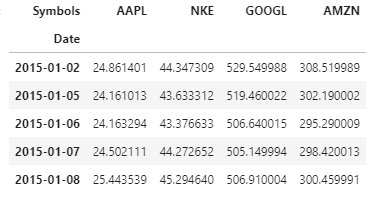
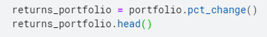
Returns: Refers to the gain or loss of our assets / portfolio for a fixed period of time. In this analysis, we make a return as the percentage change in the closing price of the asset over the closing price of the previous day. We will calculate the returns using.pct_change () function in python.

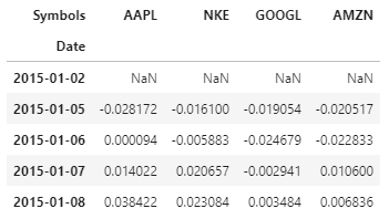
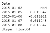
Below is the Python code to do the same and the 5 top rows (header) of returns

Note: the first row is Null if there is no previous row to facilitate the calculation of the percentage change.

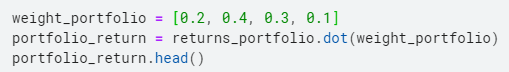
Returning a wallet is defined as the weighted sum of the returns on the portfolio assets.

To demonstrate how to calculate portfolio performance in Python, let's initialize the weights randomly (that we will then optimize). The portfolio return is calculated as shown in the code below and the portfolio returns header is also displayed:

We have seen how to calculate returns, now let's change our focus to another concept: Risk

The risk associated with assets and portfolio

The method to calculate the risk of a portfolio is written below and later we explain and give the mathematical formulation for each of the steps:

• Calculate the covariance matrix on the performance data.
• Annualize the covariance by multiplying by 252
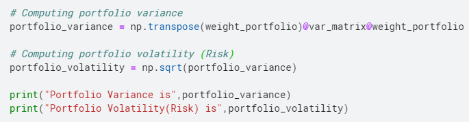
• Calculate the variance of the portfolio by multiplying it with weight vectors.
• Calculate the square root of the variance calculated above to obtain the standard deviation. This standard deviation is called the portfolio volatility..

The formula to calculate the covariance and annualize it is:

covariance = returns.cov () * 252

how is there 252 business days, we multiply the covariance by 252 to annualize it.

The variation of the portfolio, to be calculated in step 3 anterior, depends on the weights of the assets in the portfolio and is defined as:

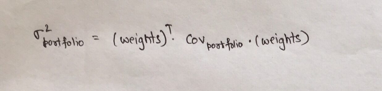
where,

• The_briefcase is the portfolio covariance matrix
• weights is the vector of weights assigned to each asset in the portfolio

Below is the approach to calculate asset risk in Python.

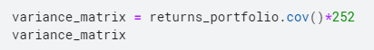
As explained above, we multiply the covariance matrix with 252, since there are 252 trading days in a year.

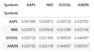
The diagonal elements of varnce_matrix represent the variance of each asset, while the terms off the diagonal represent the covariance between the two assets, for instance: the element (1,2) represents the covariance between Nike and Apple.

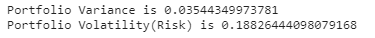
The code to calculate portfolio risk in python, whose method we saw earlier, is as shown:

Now, the task for us is to optimize the weights. Why? So that we can maximize our return or minimize our risk, And we do that using modern portfolio theory!!

Modern portfolio theory

Modern portfolio theory holds that the risk and return characteristics of an investment should not be considered alone, Rather, they should be evaluated based on how the investment affects the overall risk and return of the portfolio.. MPT shows that an investor can build a portfolio of multiple assets that will maximize returns for a given level of risk.. in addition, given a desired level of expected return, an investor can build a portfolio with the lowest possible risk. Based on statistical measures such as variance and correlation, the performance of an individual investor is less important than how it impacts the entire portfolio. [Investopedia]

This theory is summarized in the following figure. We find the frontier as shown below and maximize the expected return for the risk level or minimize the risk for a given expected return level.

Our goal is to choose the weights for each asset in our portfolio so that we maximize the expected return given a level of risk..

Mathematically, the objective function can be defined as shown below:

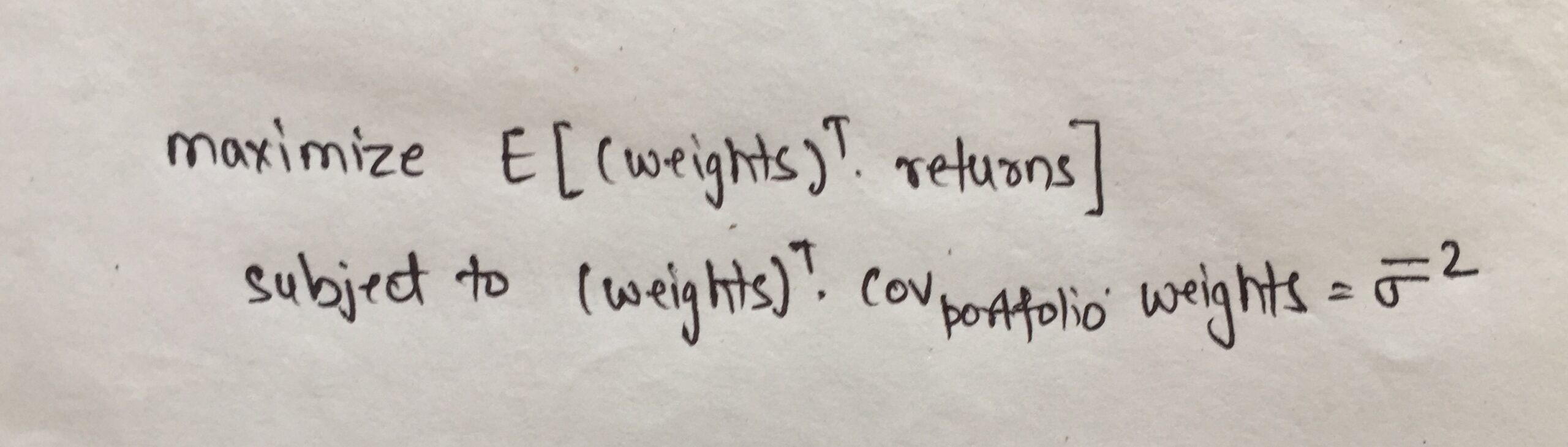
Another way of looking at the Efficient Frontier and the objective function is that we can minimize the risk given that the expected return is at least greater than the given value.. Mathematically, this objective function can be written as:

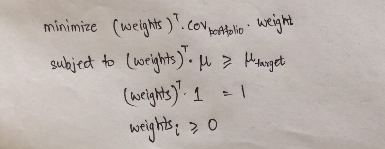
the first line represents that the objective is to minimize the variance of the portfolio, namely, in turn the volatility of the portfolio and, therefore, minimize risk.

Restricted implies that returns must be greater than a particular target return, all weights must add 1 and the weights must not be negative.

Now that we know the concept, Let's move on to the practical part now!

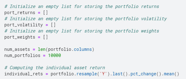
First, we create the efficient boundary by executing a loop. In every cycle, we consider a different set of randomly assigned weights for the assets in our portfolio and calculate the return and volatility for that combination of weights.

For this we create 3 empty lists, one to store returns, another to store volatility and the last to store portfolio weights.

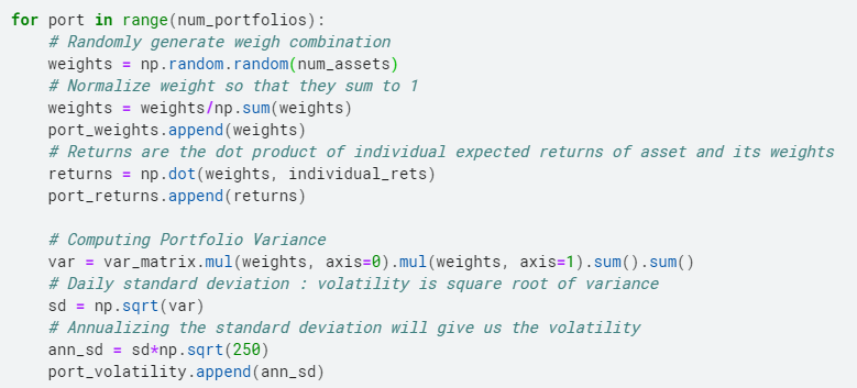
Once we have created the lists, we randomly generate the weights of our assets repeatedly, then we normalize the weighting to add 1. Then we calculate the returns in the same way we calculated above. Subsequently, we calculate the variance of the portfolio and then take the square root and then annualize it to obtain the volatility, the measure of risk for our portfolio.

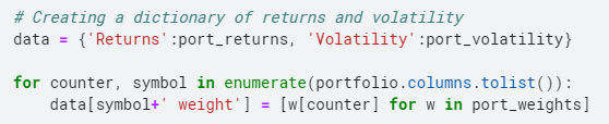
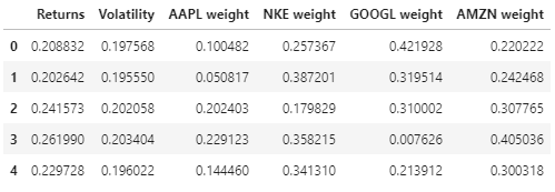
Now we aggregate the data into a dictionary and then create a data frame to see the combination of asset weights and the corresponding returns and volatility they generate.

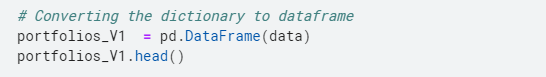
Here is the preview of the profitability data, portfolio volatility and weights.

Now we have everything with us to enter the last lap of this race and find the optimal weight set!!

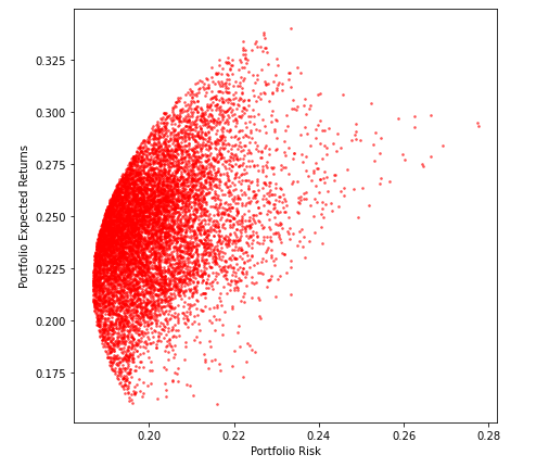
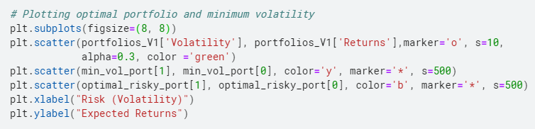
We plot the Volatility against the returns we calculated previously, this will give us the Efficient Frontier that we wanted to create at the beginning of this article.

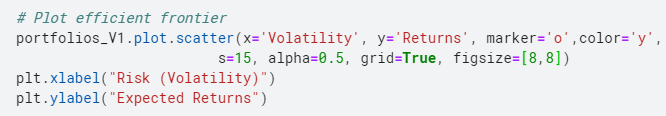
And here we go!!

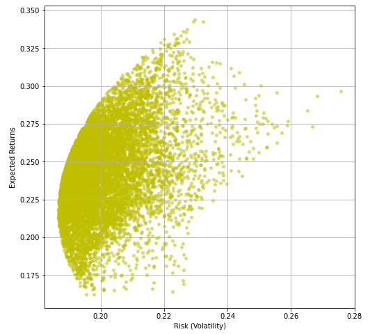
Now that we have the Efficient Frontier with us, let's find the optimal weights.

We can optimize the use of various methods as described below:

• Portfolio with minimal volatility (risk)
• Optimal portfolio (Sharpe maximum ratio)
• Maximum return at risk level; Minimal risk at an expected level of return; Portfolio with the highest Sortino ratio

In this article I will optimize through the first two approaches. In the third segment, the ‘Maximum return at a risk level’ and the ‘Minimum risk at an expected level of return’ they are quite simple, while the one based on the Sortino index is similar to the Sharpe index.

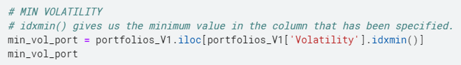
1. Minimum volatility

To find the combination of minimum volatility, we select the row in our data frame that corresponds to the minimum variance and find that row using the .idxmin function (). The code to do the same is shown below:

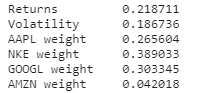
The weights we get from this are:

Now, find out where the lowest point of volatility is on the curve above. The answer is displayed at the end! But don't cheat!

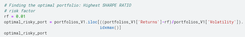
2. Higher sharpness ratio

The Sharpe index is the average return obtained in excess of the risk-free rate per unit of volatility or total risk.. The formula used to calculate the Sharpe ratio is given below:

Sharpness ratio = (R_pag – R_F)/ DAKOTA DEL ON_pag

where,

• R_pag is the return of the portfolio
• R_F is the risk-free rate
• Dakota del sur_pag is the standard deviation of the portfolio returns

The code to calculate the most optimal portfolio, namely, portfolio with the highest Sharpe index, shown below:

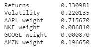
Then, Portfolio weights that give the highest Sharpe index are shown:

Find out where the highest Sharpe relationship point is on the curve above. The answer is shown below! One more time, do not cheat!

As promised here is the answer to the two questions above!!

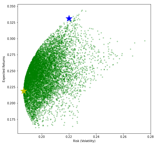
The blue star corresponds to the highest Sharpe relationship point and the yellow star corresponds to the point of minimum volatility.

Now, before finishing this article, I encourage you to find the Maximum Return portfolio at a risk level ‘and’ Minimum Risk at an Expected Profitability Level 'and mark them in the previous graph.

In addition to using the Sharpe relation, we can also optimize the portfolio using the Sortino relationship.

Giving a brief about it:

the Sortino relationship is a variation of the Sharpe index that differentiates harmful volatility from overall overall volatility by using the asset standard deviation of negative portfolio returns (downward deviation) rather than the total standard deviation of portfolio returns. The Sortino ratio takes the return on an asset or portfolio and subtracts the risk-free rate, and then divide that amount by the asset's downward drift. [Investopedia]

Sort Ratio = (R_pag – r_F)/ DAKOTA DEL OND

where,

• R_pag is the return of the portfolio
• r_F is the risk-free rate
• Dakota del surD is the standard deviation of the handicap

In case you have any trouble implementing or understanding the 3 optimization methods I described above, write me at [email protected] | [email protected] | or contact LinkedIn at https://www.linkedin.com/in/parth-tyagi-4b867452/

Note about the author: Parth Tyagi is currently studying PGDBA at IIM Calcutta, IIT Kharagpur & Indian Statistical Institute-Kolkata and has completed the B.Tech from IIT Delhi. Has ~ 4 years of work experience in advanced analytics.

Related