Principal component analysis | Guide to Principal Component Analysis

Table of Contents

• Introduction

• Smooth overview

• Cons of using PCA

• Practical example

• Conclution

Introduction

“Artificial intelligence is the latest invention humanity will need to make”. The quote definitely makes it clear that machine learning is the future and great opportunities and benefits for all. Let this be a fresh start for you to learn a really cool algorithm in machine learning.

As everybody know, we often run into the problems of storing and processing big data in machine learning tasks, as it is a time-consuming process and difficulties also arise in interpreting. Not all data characteristics are necessary for predictions. This noisy data can lead to poor performance and model overfitting. Through this article, let me introduce you to a PCA unsupervised learning technique (Principal component analysis) which can help you effectively deal with these issues to some extent and provide more accurate prediction results.

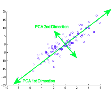
The PCA was invented in the early 20th century by Karl Pearson, analogous to principal axis theorem in mechanics and is widely used. Through this method, we actually transform the data into a new coordinate, where the one with the highest variance is the principal principal component. Thus providing us with the best possible data representations.

Soft abstract

Data with many characteristics can have correlations and duplications within it. Then, once you get the data, the main step is to clean them by removing irrelevant features and applying feature engineering techniques that can even provide better results than the original features. Principal component analysis (PCA) is one of those techniques by which dimensionality reduction is possible (linear transformation of existing attributes) and multivariate analysis. It has several advantages, including data size reduction (Thus, faster execution), better visualizations with fewer dimensions, maximize variance, reduces overfitting, etc.

The principal component actually means the direction vector sequences that differ based on the lines of best fit. It can also be stated that these components are eigenvectors of the covariance matrix. We will examine that concept below..

How do you do this? Initially, you need to find the main components from different points of view during the training phase, from those that you pick up the important and least correlated components and ignore the rest of them, thus reducing complexity. The number of principal components can be less than or equal to the total number of attributes.

Suppose that two columns X and Y are the 2 features,

XY

1 4

2 3

3 4

4 6

5 8

To mean

X ‘= 3, Y’ = 5

Covarianza

the (x, Y) = Σ (Xi – X ‘) (Yi – AND') / n – 1, where i = 1 an

C = [ the(x,x) the (x,Y) ]
[the(Y,x) the(Y,Y) ]

Similarly, for more features, we find the complete covariance matrix with more dimensions. By continuing to calculate eigenvalues, vector, etc., we can find the main components. Importing algorithms and using exact libraries makes it easy to identify components without calculations / manual operations. Note that the number of eigenvalues / Eigenvectors will give you the number of dimensions and the amount of variance associated with those components.

However, as there are numerous major components to big data, is selected primarily on the basis of which represents the greatest possible variation. As a result, the following components are also decided in decreasing order of variance of the previous components by ordering the eigenvalues, as long as these also do not have a correlation with the previous principal components. Then we discard those components with less eigenvalues / vector (less significant).

In the last step, we use feature vectors to orient the data to those represented by the principal components (Principal component analysis). This is done by multiplying the transpose of the original data set by the transpose of the feature vector.

Cons of using PCA / Disadvantages

You should be aware that data standardization (which also includes converting categorical variables to numeric) is a must before using PCA. When applying PCA, independent features become less interpretable because these main components are also not readable or interpretable. There are also chances that you will lose information during PCA.

Practical example

Now, let's see how an algorithm is implemented in a data set. I will walk you step by step through each part of the code.

Take a look at this data set. This is the famous IRIS flower dataset, containing characteristics such as sepal length, petal length, the width of the sepal and the width of the petal, and the target variable is the species. What you mean by target variable is the value / class you need to predict, which in this case is the species class to which the flower belongs.

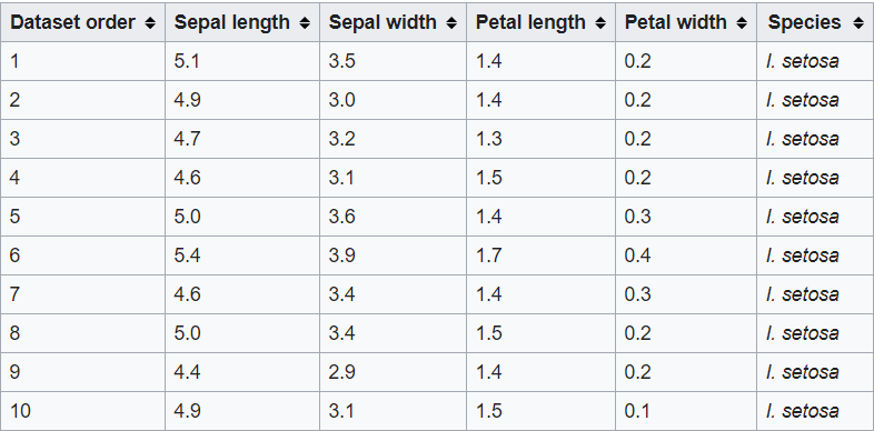
source: Wikipedia

Importing data sets and basic libraries

First, let's start by importing the necessary libraries,

import numpy as np 
import pandas as pd 
import matplotlib.pyplot as plt
from sklearn.datasets import load_iris

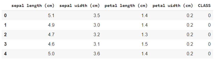
Load the data and display the names of the characteristics and classes for your understanding,

iris = load_iris()
#Feature names and Encoding of target variables
print(iris.feature_names)
print(iris.target_names)
data = pd.DataFrame(iris.data)
data.columns = iris.feature_names
data['CLASS'] = iris.target
data.head()

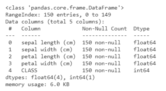
The following code snippet helps you get an analysis of the data, namely how many variables are categorical and how many are numerical. What's more, it is clear below that all rows are not null, in case of null objects, we get the count and rows / columns in which they are present. This helps us go through the preprocessing steps to clean up the data.

data.info()

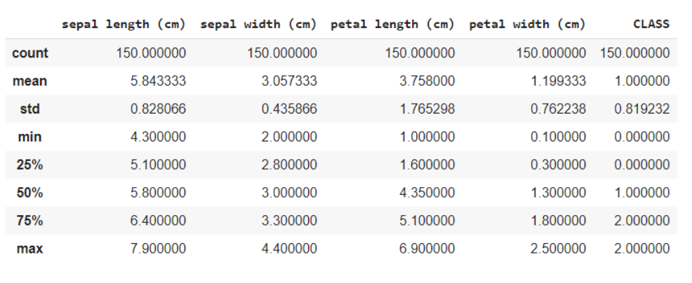
The data.describe function () generally provides a statistical description of the dataset. These could be beneficial in many ways, you can use this data to fill in missing values ​​or create a new characteristic, and many more.

data.describe()

Here you are dividing the data into the characteristics and the target variables as X and and respectively. And when using the shape method, knows that the data has 150 rows and 5 columns in total, of which 1 column is your target variable and others 4 are the characteristics / attributes.

x = data.iloc[:,:4]  #features
y = data.iloc[:,4] #target
x.shape, y.shape

Out of: ((150, 4), (150,))

Since all characteristics are numeric, it is easy for the model for training. If the data contained categorical variables, we must first convert them to numeric, since the machines / computers can handle numbers better.

PCA Library Import

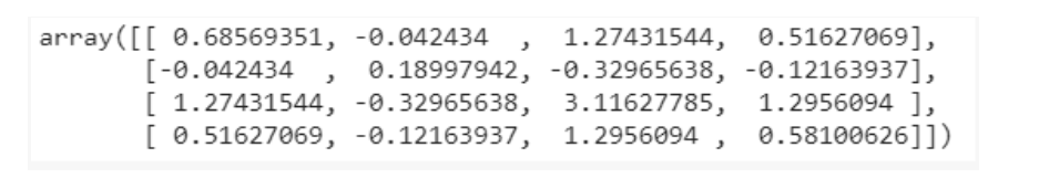
from sklearn.decomposition import PCA
pca = PCA()
X = pca.fit_transform(x)
pca.get_covariance()

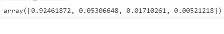
explained_variance=pca.explained_variance_ratio_
explained_variance

Visualizations

with plt.style.context('dark_background'):
    plt.figure(figsize=(6, 4))
    plt.bar(range(4), explained_variance, alpha=0.5, align='center',
            label="individual explained variance")roduction
    plt.ylabel('Explained variance ratio')
    plt.xlabel('Principal components')
    plt.legend(loc ="best")
    plt.tight_layout()

From the visualizations the intuition is obtained that there are mainly only 3 components with significant variance, Thus, we select the number of principal components as 3.

pca = PCA(n_components=3)
X = pca.fit_transform(x)

Split train test

The train testing division is a common method of training and evaluation. As usual, predictions on the trained data themselves can lead to overfitting, thus giving bad results for unknown data. In this case, by dividing the data into training and test sets, you train and then predict using the model in 2 different sets, thus solving the problem of overfitting.

from sklearn.model_selection import train_test_split
X_train, X_test, y_train, y_test = train_test_split(X, Y, test_size = 0.3, random_state=20, stratify=y)

Model training

Our goal is to identify the class / species to which the flower belongs given some of its characteristics. Therefore, this is a classification problem and the model we use uses K nearest neighbors.

from sklearn.neighbors import KNeighborsClassifier
model = KNeighborsClassifier(7)
model.fit(X_train,y_train)
y_pred = model.predict(X_test)

Predictions

from sklearn.metrics import confusion_matrix
from sklearn.metrics import accuracy_score
cm = confusion_matrix(y_test, y_pred)  #confusion matrix
print(cm)
print(accuracy_score(y_test, y_pred))

The confusion matrix will show you the false positive count, false negatives, true positives and true negatives.

The precision score will tell you how effective our model has been in providing predictions for new data. The 97% it's a very good score, and that is why we can say that ours is a good model.

You can see the complete code at this google collaboration planned.

Conclution

I really hope you have had intuition about PCA and are also familiar with the example discussed above. It is not that complex to digest, just stay focused. Make sure to read this one more time if you find it useful and develop the algorithm yourself to understand it better..

Have a nice day !! 🙂

Related