Random forests in machine learning

This article was published as part of the Data Science Blogathon.

Introduction

TIGHTEN FOR IMPACT! CLAMP! CLAMP! CLAMP!

¡¡¡UPS!!! Our plane has crashed, but luckily we are all safe. We are data scientists, so we want to open the black box and see what random things have been registered inside. Yes, let's move on to our topic.

What are random forests?

You must have solved at least once a probability problem in your high school in which you were supposed to find the probability of getting a ball of a specific color from a bag containing balls of different colors., given the number of balls of each color. Random forests are simple if we try to learn them with this analogy in mind.

The random forests (RF) they are basically a bag containing n decision trees (DT) which have a different set of hyperparameters and are trained on different subsets of data. Let's say I have 100 decision trees in my random forest bag! As i just said, these decision trees have a different set of hyperparameters and a different subset of training data, so the decision or prediction given by these trees can vary greatly. Let us consider that I have somehow trained all of these 100 trees with their respective subset of data. Now I will ask the hundred trees in my bag what is their prediction on my test data. Now we just need to make a decision on an example or a test data, we do it by means of a simple vote. We follow what most trees have predicted for that example.

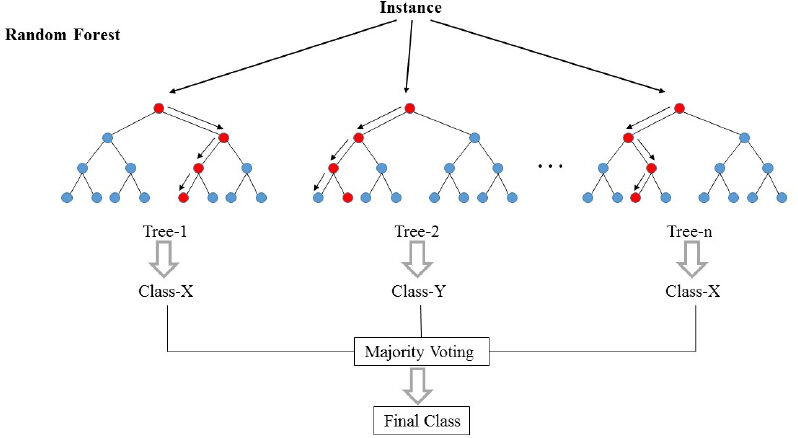
In the picture above, we can see how an example is classified using n trees where the final prediction is made by taking a vote from all n trees.

In the language of machine learning, RFs are also called assembly or bagging methods. I think the word bag could come from the analogy we just discussed!!

Let's get a little closer to ML Jargons !!

The random forest is basically a supervised learning algorithm. This can be used for both regression and classification tasks. But we will discuss its use for classification because it is more intuitive and easier to understand.. The random forest is one of the most used algorithms due to its simplicity and stability.

While building subsets of data for trees, the word “random” enters to scene. A subset of data is created by randomly selecting x number of features (columns) y y number of examples (rows) from the original data set of n characteristics and m examples.

Random forests are more stable and reliable than just a decision tree. This is simply saying that it is better to vote for all cabinet ministers rather than simply accepting the decision given by the prime minister..

As we have seen that random forests are nothing more than the collection of decision trees, knowledge of the decision tree becomes essential. So let's dive into decision trees.

What is a decision tree?

In very simple words, it's a “Set of rules” created by learning from a data set that can be used to make predictions about future data. We will try to understand this with an example.

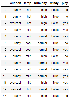
Here is a small simple data set. In this data set, the first four characteristics are independent characteristics and the last four are dependent characteristics. The independent characteristics describe the weather conditions on a given day and the dependent characteristic tells us if we were able to play tennis that day or not..

Now we will try to create some rules using independent characteristics to predict dependent characteristics. Just by observation, we can see that if Outlook is cloudy, the game is always yes, regardless of other characteristics. Similarly, we can create all the rules to fully describe the data set. Here are all the rules.

1. • R1: And (Outlook = Sunny) Y (Humidity = High) Then Play = No
   • R2: And (Outlook = Sunny) Y (Humidity = Normal) Then Play = Yes
   • R3: And (Outlook = Cloudy) Then Play = Yes
   • R4: And (Outlook = Rain) Y (Wind = Strong) Then Play = No
   • R5: And (Perspective = Rain) Y (Wind = Weak) Then Pay = Yes

We can easily convert these rules into a tree diagram. Here is the tree chart.

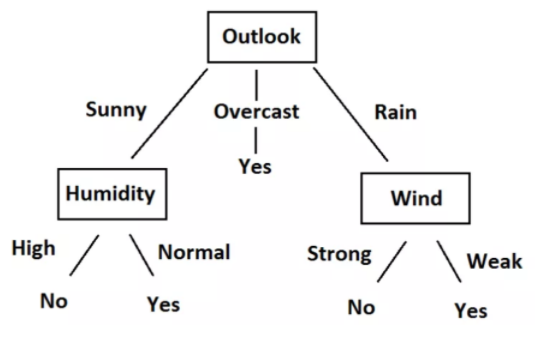
By looking at the data, the rules and the tree, You will understand that we can now predict whether we should play tennis or not, given the climate situation based on independent characteristics. All this process of creating rules for a given data is nothing more than the training of the decision tree model.

We could set rules and make a tree just by looking here because the dataset is so small. But, How do we train the decision tree on a larger data set? For that, we need to know a little math. Now we will try to understand the mathematics behind the decision tree.

Mathematical concepts behind the decision tree

This section consists of two important concepts: Entropy and Information Gain.

Entropy

Entropy is a measure of the randomness of a system. The entropy of the sample space S is the expected number of bits needed to encode the class of a randomly drawn member of S. Here we have 14 rows in our data, hence 14 members.

Entropy E (S) = -∑p (x) * log₂(p (x))

The entropy of the system is calculated using the above formula, where p (x) is the probability of obtaining the class x of those 14 members. We have two classes here, one is Yes and the other is No in the Play column. Have 9 Yes, and 5 Not in our dataset. Then, the calculation of the entropy here will be as follows

E (S) = -[p(Yes)*log(p(Yes))+ p(No)*log(p(No))]= -[(9/14)*log((9/14))+ (5/14*log((5/14)))]= 0,94

Information gain

The information gain is the amount in which the Entropy of the system is reduced due to the division that we have made. We have created the tree using observations. But, How come we decided that we should split the data first based on Outlook and not any other function? The reason is that this division was reducing entropy by the maximum amount, but we did it intuitively in the example above.

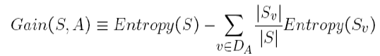
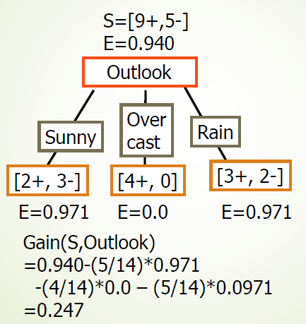
The division of the tree above shows us that 9 Yes, and 5 They have not been divided as (2 Y, 3 N), (4 Y, 0 N), (3 Y, 2 N), when we do the division according to perspective. The E values ​​below each division show entropy values ​​considering themselves as a complete system and using the entropy formula above. Later, we have calculated the information gain for the prospect split using the gain formula above.

Similarly, we can calculate the information gain for each feature division independently. And we get the following results:

• • Gain (S, Outlook) = 0,247
  • Gain (S, humidity) = 0,151
  • Gain (S, wind) = 0.048
  • Gain (S, temperature) = 0.029

We can see that we are getting the maximum information gain by splitting the Outlook function. We repeat this procedure to create the entire tree. I hope you enjoyed reading the article. If you like the article, share it with your colleagues and friends. Happy reading!!!

Related